library("spatstat")
library("inlabru")
library("ggplot2")
library("tmap")
library("raster")
library("rgeos")
library("INLA")
library("sf")Inference in Point Processes
In this tutorial, we will use the following R packages.
Point process
Let x \in \mathcal{D} \subseteq \mathbb{R}^n, n \in \{1, 2, \cdots\}, such that \mathcal{D} is the domain. Then, a point process \xi is defined as a locally finite random subset of \mathcal{D}; that is, \mathcal{N}(D) := \#(\xi \cap \text{D}) is finite for all bounded subsets \text{D} \subseteq \mathcal{D}, where \#(\text{A}) denotes de cardinality of \text{A}.
As a note, a point process is random mechanism whose outcome is a point pattern.
Intensity
For a point process, we may define an intensity function as follows
Let \lambda: \mathcal{D} \rightarrow [0, +\infty), such that \int_{D}\lambda(x)dx < +\infty, for all bounded \text{D} \subseteq \mathcal{D}. \lambda(x) is the intensity function of a point process \xi, if \mathbb{E}[\mathcal{N}(D)] = \int_{\text{D}}\lambda(x)dx, ~ \text{D} \subseteq \mathcal{D}.
If \lambda(x) = \lambda, \forall x, that is, if it is a constant function, notice that \mathbb{E}[\mathcal{N}(D)] = \lambda \cdot |\text{D}|. In that case, \lambda denotes the average number of points per unit area.
Also, the intensity function is closely related to the probability density.
If \xi is a point process with intensity function \lambda(x) defined on \mathcal{D}, then each individual point inside \mathcal{D} has probability density f(x) = \frac{\lambda(x)}{\Lambda_{\mathcal{D}}}, where \Lambda_{\mathcal{D}} = \int_{\mathcal{D}}\lambda(x)dx.
Using spatstat we can generate a point pattern containing n independent, identically distributed random points with intensity f using the rpoint() function.
f <- function (x, y) { (x ** 2 + y ** 2) }
x <- seq(-1, 1, 0.05)
y <- seq(-1, 1, 0.05)
z <- outer(X = x, Y = y, FUN = f)
w <- owin(xrange = c(-1, 1), yrange = c(-1, 1)) # Area: (2 units x 2 units)

pp <- rpoint(n = 200, f = f, win = w)

par(mfrow = c(1, 2))
persp(x, y, z, theta = 30)
plot(pp, main = "")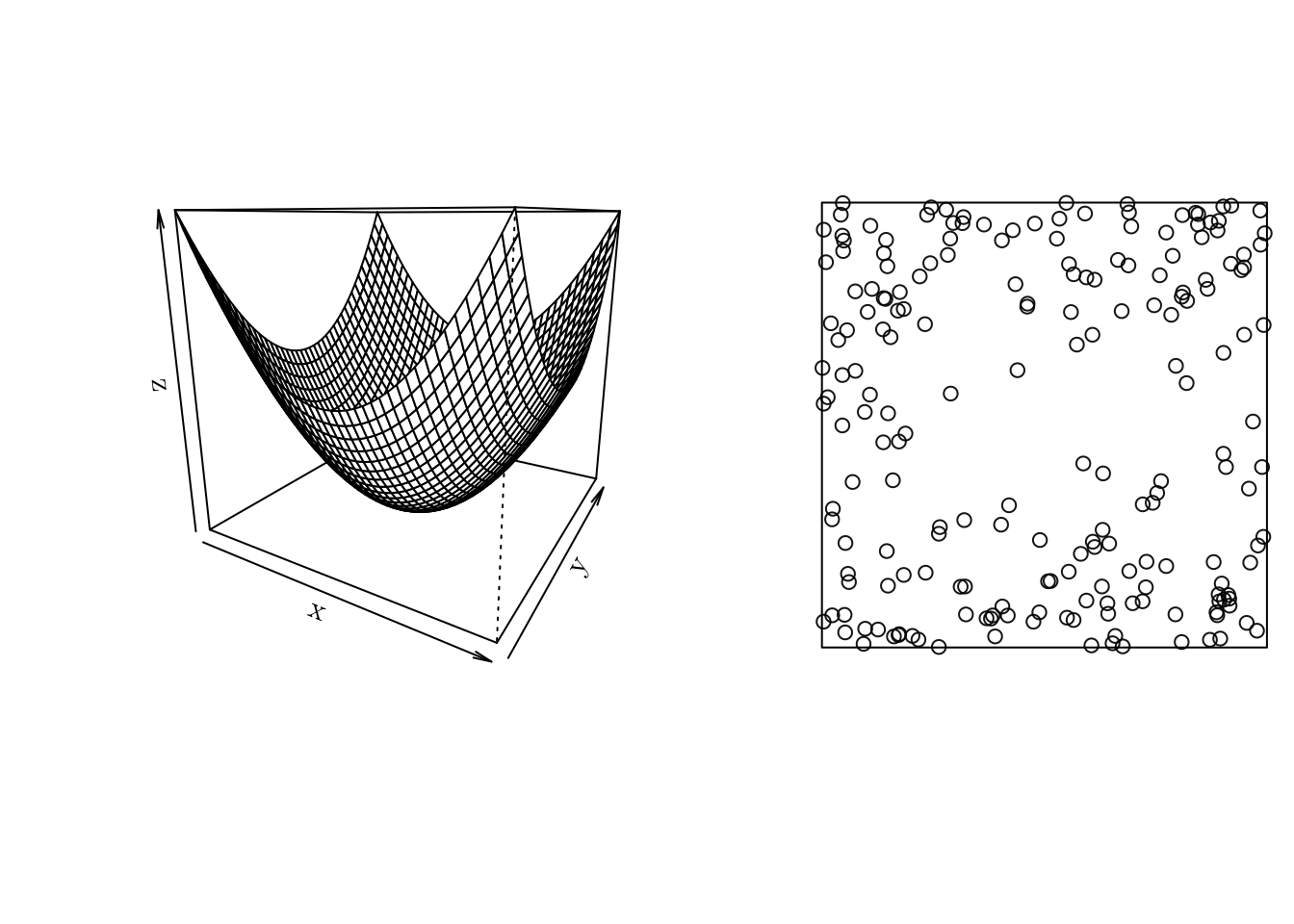
Poisson Point Process
A point process \xi defined on \mathcal{D} is a Poisson point process with intensity function \lambda(x) if the following properties are satisfied
For any bounded \text{D} \subseteq \mathcal{D}, \mathcal{N}(\text{D}) \sim \text{Poisson}(\int_{\text{D}}\lambda(x)dx).
For any bounded \text{D} \subseteq \mathcal{D} and n \in \mathbb{N}, conditional on \mathcal{N}(\text{D}) = n, the events \xi \cap \text{D} are independent with intensity proportional to \lambda(x).
As a note, it \lambda(x) = \lambda, \forall x, then \xi is a homogeneous Poisson process; otherwise, it is a non-homogeneous Poisson process.
Homogeneous Poisson process
We can manually simulate a homogeneous Poisson process as follows
- Determine \mathcal{N}(D), for some D \subseteq \mathcal{D}.
- Simulate the number of events n from a Poisson(\lambda\cdot|D|).
- Obtain the location of the n events by simulating from an uniform distribution.
sim.HPP <- function (lambda, max = 1, min = 0, ...) {
  m <- lambda * (max - min)
  N <- rpois(1, lambda = m)
  sort(runif(N, min = min, max = max))
}

hpp <- sim.HPP(lambda = 0.5, max = 100, min = 0)
print(hpp)
[1] 0.3535495 0.5396310 5.5676715 10.3492299 11.1476796 14.4515851
[7] 14.9180392 15.9673980 17.4775137 19.1189961 19.6719169 19.9752943
[13] 22.1834201 22.2928340 24.2387337 25.0736451 26.7346206 32.7452220
[19] 41.6347296 43.4830146 43.5288069 43.8059504 44.7422891 49.2827306
[25] 51.4434260 57.4189733 57.7254297 57.7635149 58.9999127 59.8600273
[31] 60.8599697 61.2403756 61.6342769 68.0476603 72.9181244 73.6506027
[37] 74.4836050 75.3390585 76.2458188 81.5512829 85.0963224 90.6697583
[43] 91.9029311 95.1212361 95.9875866 99.2158440 99.7424144 99.7688745print(length(hpp))[1] 48# Plot 1D PP
plot1D.pp <- function (pp, xlim = NA, ...) {
par(mfrow = c(1, 1))
if (is.na(xlim)) { xlim <- c(floor(min(pp)), ceiling(max(pp))) }
plot(x = NA, xlab = "", ylab = "", xlim = xlim, ylim = c(0, 1), axes = FALSE, frame = FALSE, asp = diff(xlim) * 0.1)
arrows(x0 = pp, y0 = 1, x1 = pp, y1 = 0)
axis(1, pos = 0)
}
plot1D.pp(hpp)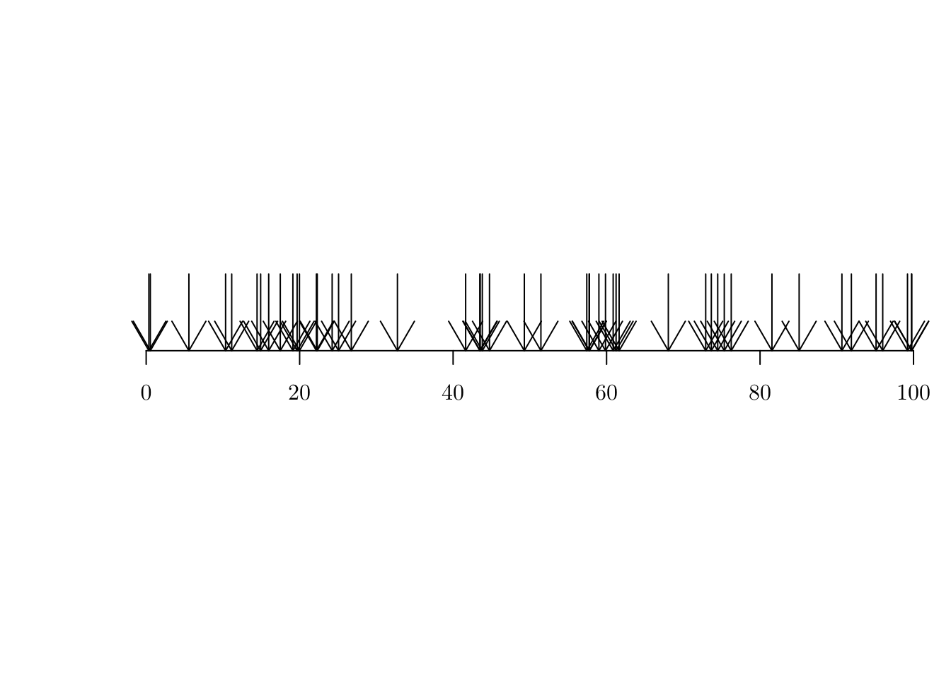
An unbiased estimator for \lambda in a homogeneous Poisson process is \hat{\lambda} = \frac{\#(x)}{|D|}, where \mathbf{x} is the point pattern data set, and D is the observed in a window.
(lambda_hat <- length(hpp) / 100)[1] 0.48Non-homogeneous Poisson process
To simulate from a non-homogeneous Poisson process, we can use the thinning approach (Lewis and Shedler, 1979).
- Find \max(\lambda(x)), i.e., the maximum of \lambda(x) in \mathcal{D}.
- Simulate a homogeneous Poisson process with \lambda = \max(\lambda(x) \cdot |D|).
- Accept each event with probability \lambda(x_i)/\max(\lambda(x)).
For example, let \lambda(x) = \exp(\beta_0 + \beta_1 \cdot x), such that \beta_0 = -1 and \beta_1 = 0.015.
l <- function(x, par, log = FALSE, ...) {
  eta <- par[1] + par[2] * x
  if (log) { res <- eta } else { res <- exp(eta) }
  res
}

pts <- seq(0, 100, 0.1)
par <- c(-1, 0.015)
plot(x = pts, y = l(pts, par), type = "l", xlab = "x", ylab = "y")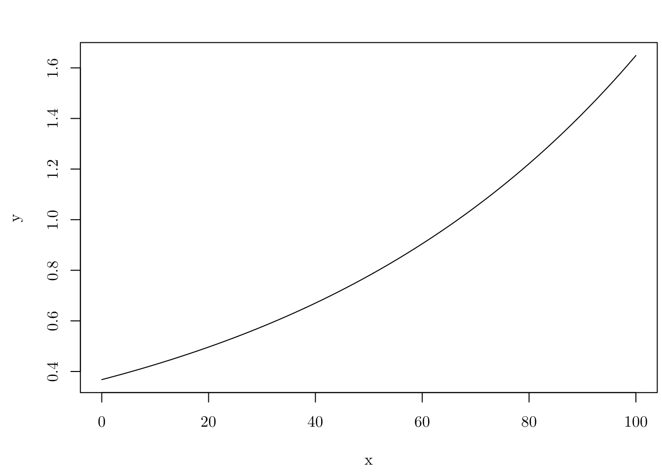
In that case, \mathbb{E}[\mathcal{N}(D)] = 85, such that D = [0, 100].
integrate(l, lower = 0, upper = 100, par = par)85.38946 with absolute error < 9.5e-13sim.NHPP <- function (par, FUN, max = 1, min = 0, ...) {
max_lb <- optimize(FUN, c(min, max), par = par, maximum = TRUE)$objective
lambda <- max_lb * (max - min)
# As in `sim.IPP()`
N <- rpois(1, lambda = lambda)
pts <- sort(runif(N, min = min, max = max))
# Accept or reject
p.accept <- FUN(pts, par) / max_lb
pp <- pts[runif(length(pts)) <= p.accept]
attributes(pp) <- list(simulated = length(pts), accepted = length(pp), rate = length(pp) / length(pts))
pp
}
nhpp <- sim.NHPP(par = par, FUN = l, max = 100, min = 0)
print(unlist(attributes(nhpp))) simulated accepted rate
143.0000000 84.0000000 0.5874126 plot1D.pp(nhpp)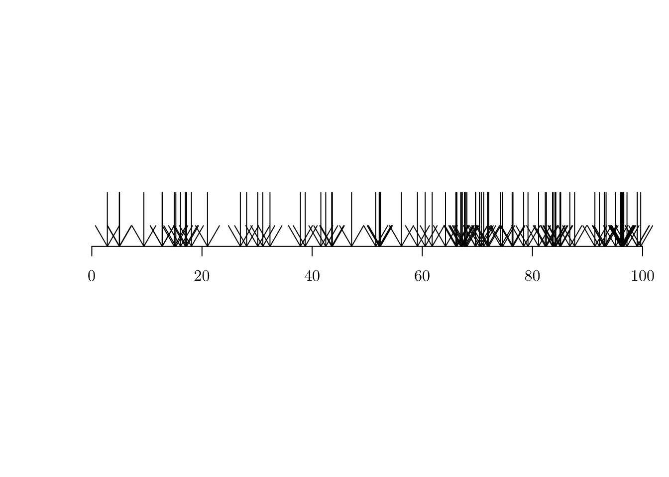
Likelihood function
The likelihood function of a point process is obtained based on the density function of the two observed variables, namely the number of events \mathcal{N} and the locations \{x\}.
For a Poisson process, we have that \mathcal{N}(D) \sim \text{Poisson}(\int_D\lambda(x)dx) and, for each x, \mathbb{P}(x_i) = \lambda(x_i) / \int_D\lambda(x)dx. Therefore, \begin{align*} L(\theta) &= \frac{e^{-(\int_D\lambda(x)dx)}(\int_D\lambda(x)dx)^N}{N!} \prod_{i = 1}^N \frac{\lambda(x_i)}{\int_D\lambda(x)dx} \\ &\propto e^{-(\int_D\lambda(x)dx)}\prod_{i = 1}^N\lambda(x_i), \end{align*} where N is a a realization of \mathcal{N}(D). The log-likelihood is given by \begin{align*} \ell(\theta) \propto \sum_{i = 1}^{N}\log(\lambda(x_i)) - \int_D\lambda(x)dx. \end{align*}
For a homogeneous Poisson process, \begin{align*} \ell(\lambda) &\propto N \log(\lambda) - \lambda\cdot|D| \\ \hat{\lambda} &= \frac{N(D)}{|D|}. \end{align*}
However, for a non-homogeneous Poisson process, the MLE for will depend of the form of \lambda(x). In our previous example \begin{align*} \ell(\beta_0 + \beta_1) \propto \sum_{i = 1}^N\log(\beta_0 + \beta_1x_i) - \int_D\beta_0 + \beta_1x dx. \end{align*} Although, in some cases it is possible to have a closed-form solution for (\hat{\beta}_0, \hat{\beta}_1)^{\top}, let us compute them numerically.
Example
Let us implement the log-likelihood function as before
lik.NHPP <- function (par, FUN, pp, max = 1, min = 0, ...) {
  int.l <- integrate(FUN, low = min, upp = max, par = par)$value
  sum.t <- sum(FUN(x = pp, par = par, log = T))
  -(sum.t - int.l)
}

initial_values <- c(0, 0)
(theta_hat <- optim(par = initial_values, fn = lik.NHPP, FUN = l, pp = nhpp, min = 0, max = 100)[1:2])
$par
[1] -1.0336698 0.0152766
$value
[1] 90.92931Hypothesis test
We can visually inspect whether the point pattern seemed to be sampled from a (non-)homogeneous process by counting the number of events by interval.
L  <- psp(x0 = 0, y0 = 0, x1 = 100, y1 = 0, owin(c(0, 100), c(-5, 5)))
pp <- as.ppp(cbind(c(nhpp), 0), W = L)

q <- quadratcount(X = pp, nx = 8, ny = 1)
plot(q, main = "")
Alternatively, we can conduct a hypothesis test. In particular, we test the null hypothesis that the data pattern is a realization of Complete Spatial Randomness”; i.e., uniform Poisson point process.
ts <- quadrat.test(X = pp, nx = 8, ny = 1)
ts
    Chi-squared test of CSR using quadrat counts

data:  pp
X2 = 22.286, df = 7, p-value = 0.004535
alternative hypothesis: two.sided

Quadrats: 8 by 1 grid of tiles
In the case of nhpp (known to be a realization from non-homogeneous process), at a 5% confidence level, we reject the null hypothesis data pattern is a realization of “Complete Spatial Randomness”.
Cox Process
As a generalization of a Poisson process, we can define a Cox process. In a nutshell, a Cox process allows the modelling of the non-observable spatial heterogeneity.
A Cox process can be seen as a doubly stochastic process. \xi is a Cox process driven by \Lambda(x) if
\{\Lambda(x); x \in \mathcal{D}\} is a non-negative valued stochastic process.
Conditional on \{\Lambda(x) = \lambda(x); \mathbf{x} \in \mathcal{D}\}, \xi is a Poisson process with intensity function \lambda(x).
A particular case of a Cox process, named log-Gaussian Cox process, can be constructed by setting \log\{\Lambda(x)\} = \mu^{\star}(x) + \zeta(x), such that \mu(x) = \exp\{\mu^{\star}(x)\} is possibly interpreted as the mean structure of \Lambda(x), and \zeta(x) is a stationary Gaussian process, such that \mathbb{E}(\zeta(x)) = -\sigma^2/2, \forall x, and \text{Cov}(\zeta(x_1), \zeta(x_2)) = \phi(h) = \sigma^2 \rho(h), where h = ||x_1 - x_2|| and \sigma^2 is the variance of \zeta(x) .
For instance, the correlation structure can be set as a Matérn model, that is, \rho(h) = \frac{1}{2^{\nu - 1}\Gamma(\nu)}(\kappa \cdot h)^{\nu} \,\text{K}_{\nu}(\kappa \cdot h), such that \nu and \kappa are unknown parameters, and \text{K}_{\nu}(\cdot) is a modified Bessel function of 2^{\text{nd}} order.
INLA and R-INLA
To fit a LGCP model, we will use the Integrated Nested Laplace Approximation, INLA (Rue et al., 2009), implemented in the R-INLA package.
In a nutshell, INLA is a method for approximating Bayesian inference in latent Gaussian models. In particular, it can be used to fit models of the form \begin{align*} y_i|S(x_i), &\theta \sim \pi(y_i|S(x_i), \theta), \text{ for } i \in \{1, \cdots, n\} \\ S(x)|\theta &\sim \text{Normal}(\mu(\theta), Q(\theta)^{-1}) \\ \theta &\sim \pi(\theta), \end{align*} where y = (y_1, \ldots, y_n) is the vector or observed values, x = (x_1, \ldots, x_n) is a Gaussian random field, and \theta = (\theta_1, \ldots, \theta_k), for some k \in \mathbb{N}, is a vector of hyperparameters. \mu(\theta) and Q(\theta) represent the mean vector and the precision matrix, respectively.
Fitting a LGCP with R-INLA
Although we can use a Stochastic Partial Differential Equation (SPDE)-approach to fit LGCP models using INLA (Simpson et al., 2016), we will consider a partition of \mathcal{D} given by cells c_{i, j}, for some set of index (i, j).
First, recall that if \xi is a LGCP, then the mean number of events in a cell c_{ij} is given by the integral of the intensity over the cell, that is, \int_{c_{i,j}}\Lambda(x)dx. Then, for sufficiently small cells, such an integral can be approximated by |c_{i,j}|\Lambda(x), where |c_{i, j}| is the area of the cell c_{i, j}.
Thus, conditional on the latent Gaussian field \zeta(x), the number of locations in the grid cell c_{i, j}, \forall i, j, are independent and Poisson distributed as follows \mathcal{N}(c_{ij})|\zeta(x) \sim \text{Poisson}(|c_{i, j}| \cdot \Lambda(x)), where \zeta(x) is a Gaussian field.
This approach is well documented in Moraga, 2020.
Example 1
For the first example, we will analyze the spatial locations of cases of lung cancer in chorley (from spatstat.data). The data give the precise domicile addresses of new cases of cancer of the larynx (58 cases) and cancer of the lung (978 cases), recorded in the Chorley and South Ribble Health Authority of Lancashire (England) between 1974 and 1983.
print(chorley)Marked planar point pattern: 1036 points
Multitype, with levels = larynx, lung
window: polygonal boundary
enclosing rectangle: [343.45, 366.45] x [410.41, 431.79] kmplot(chorley, cols = c("red", rgb(0, 1, 0, 0.5)), pch = c(19, 4), cex = 0.75, main = "Cancer cases")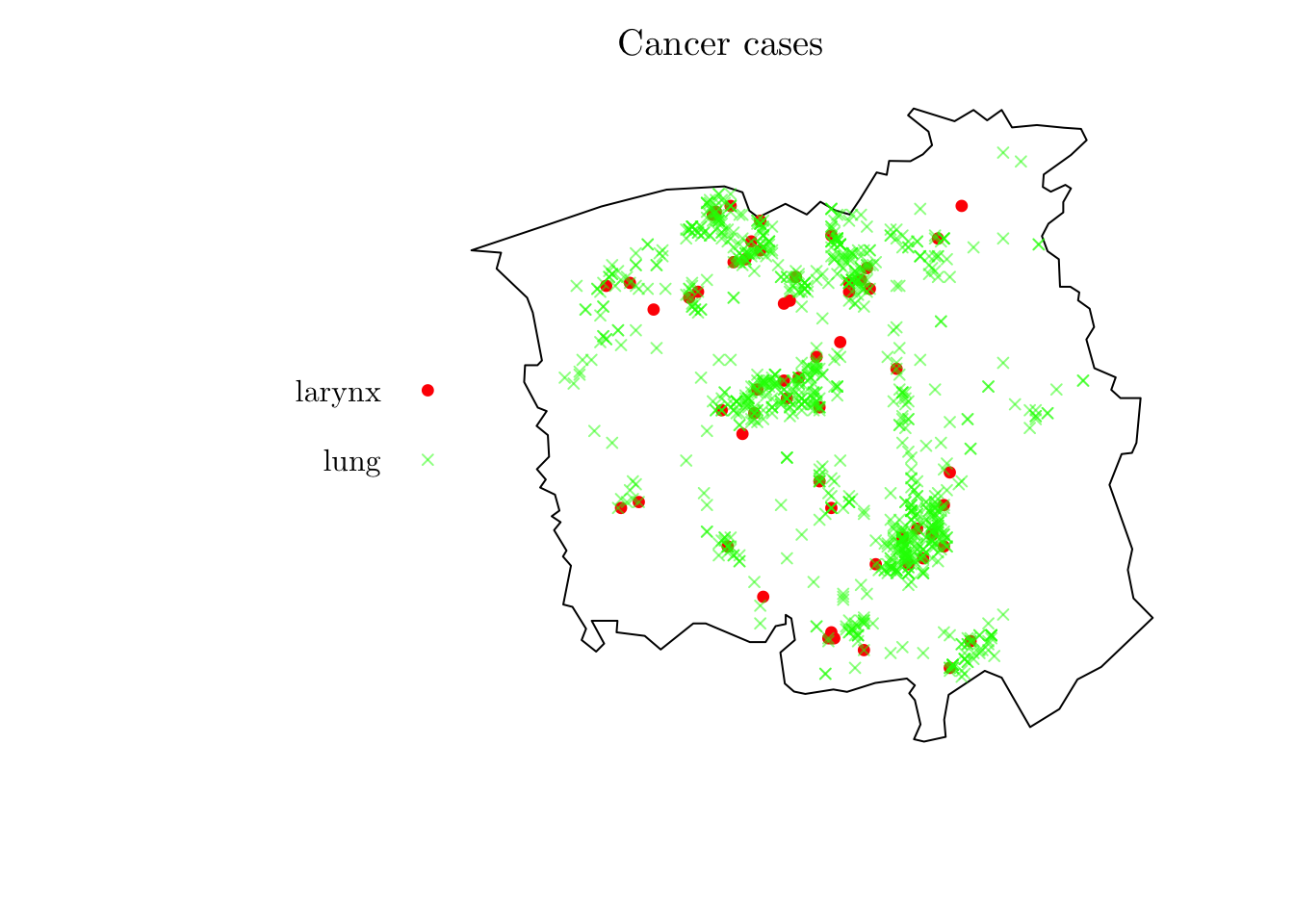
lung <- chorley[chorley$marks == "lung"]
lung <- ppp(x = lung$x, y = lung$y, window = lung$window)

plot(lung, cols = "green", pch = 4, cex = 0.75, main = "Lung-cancer cases")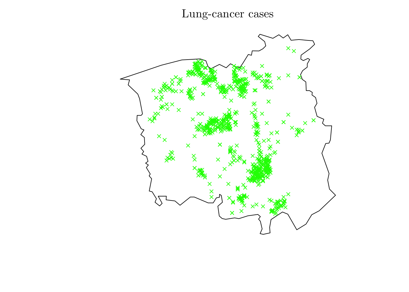
Let us start by creating a grid based study area.
resolution <- 0.5
map <- as(st_as_sf(lung$window), "Spatial") # Convert it to a `SpatialPolygonsDataFrame` object
map$cancer <- "lung"
plot(map)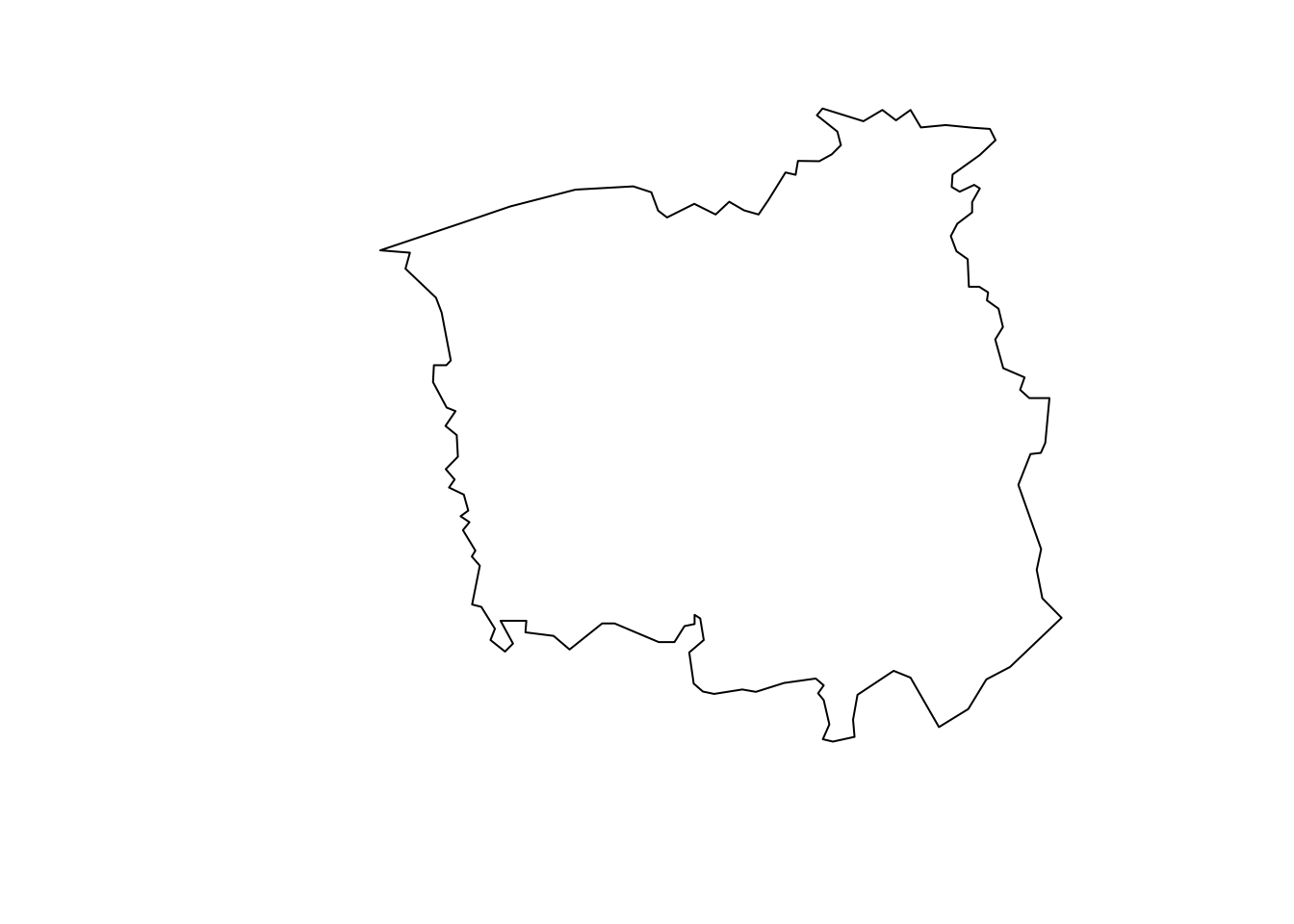
r <- raster(map, resolution = resolution) # Create a `raster` object based on the map and resolution
(n_row <- nrow(r))
[1] 43(n_col <- ncol(r))[1] 46Now, we have to count the number of observations within all cells and save it on the r object. To do so, we can create a SpatialPoints object based on the observations locations and use the cellFromXY() to count the number of points in each cell.
r[] <- 0 # Set all `NA` to `0`
dpts <- SpatialPoints(cbind(rev(lung$x), rev(lung$y))) # Convert the locations to a `SpatialPoints` object

(tab <- table(cellFromXY(r, dpts)))
 128  176  247  248  292  293  294  301  307  337  338  339  341  342  343  347
   1    1    2    1    4    9    5    3    1    4    3   12    2    9    1    5
 348  349  383  384  385  386  387  388  389  393  397  398  399  400  404  426
   2    2    6    6    6    5    2    6    3   13    5    2    2    7    1    3
 427  432  433  434  435  439  440  441  444  445  446  448  453  470  472  473
   3    2   11   13    4    8    7    5    3    4    3    1    2    3    2    2
 478  479  480  481  482  484  485  486  487  488  491  492  493  514  515  516
   2    8    1    1    1    1    3    8    7    2    1    2    1    1    1    5
 517  518  521  522  527  528  529  530  531  532  533  535  537  538  539  561
   3    1    2    1    2    7    7    2    2   14    7    2    1    1    1    3
 564  566  567  568  570  574  575  578  579  606  607  613  614  621  624  625
   2    1    4    1    2    2    8    2    6    2    3    3    6    1    2    1
 654  656  668  673  676  699  700  701  744  745  749  753  754  760  761  765
   2    1    1    2    2    3    2    1    1    1    1    1    1    2    3    2
 767  790  802  803  805  806  811  818  835  844  847  848  849  850  851  852
   1    2    1    3    6   11    3    1    2    1    1   13   10    6   11    1
 853  857  860  863  868  870  891  892  893  894  895  896  897  898  899  903
   4    1    1    2    1    2    2    9   10    3    5    8   11   11    1    1
 904  911  937  938  939  940  941  942  943  944  950  954  958  959  975  982
   8    1    5    3    4    9    4    4    1    5    4    2    1    6    1    1
 985  986  995  996  999 1004 1022 1042 1043 1044 1046 1073 1080 1083 1088 1091
   3    1    2    1    1    1    1    1    1    1    2    1    3    1    2    1
1128 1129 1134 1136 1161 1162 1166 1174 1175 1179 1180 1181 1182 1183 1184 1206
   5    1    3    1    2    1    1    3    2    1    3    1    1    2    1    1
1207 1208 1212 1217 1221 1222 1226 1227 1228 1266 1269 1271 1272 1273 1274 1304
   3    1    1    1    4    6    5    6   10    2    2    2    9    7   11    2
1306 1311 1317 1318 1319 1320 1321 1351 1352 1362 1363 1364 1365 1366 1367 1397
   3    1    4   14    5   19    2    2    7    2    9   19    7   13    2    1
1398 1399 1402 1408 1409 1410 1411 1412 1446 1450 1454 1455 1456 1457 1498 1499
   2    3    1    2   12   19    6    2    1    1    3    8    5    4    2    2
1502 1538 1544 1584 1588 1590 1591 1592 1599 1600 1635 1636 1637 1642 1643 1644
   1    1    1    1    2    3    7    1    1    1    2    8    4    1    1    5
1645 1646 1683 1685 1686 1687 1690 1691 1692 1728 1735 1736 1772 1782
3 6 1 1 1 1 6 5 1 1 10 7 2 2 r[as.numeric(names(tab))] <- tab # Assign the number of observed events to the `raster` object
plot(r)
plot(map, add = T)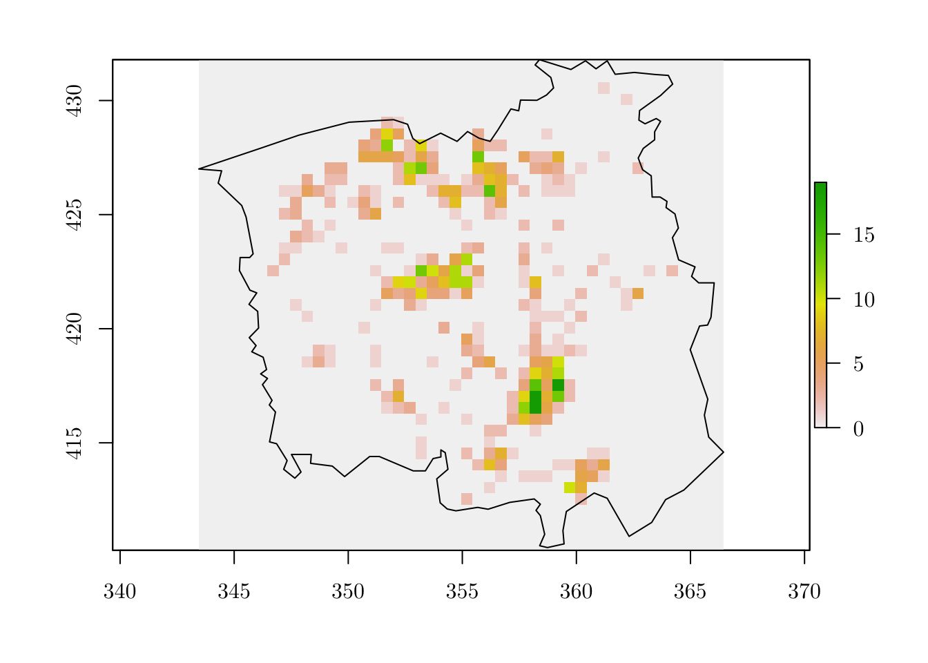
Then, we can create a grid variable based on the raster object.
grid <- rasterToPolygons(r) # Convert it to a `SpatialPolygonsDataFrame` object

grid <- grid[as.vector(matrix(1:nrow(grid), nrow = n_row, ncol = n_col, byrow = T)), ] # Rearrange the indices numbering

grid$id <- 1:nrow(grid)
grid$Y <- grid$layer
grid$cellarea <- resolution * resolution
plot(grid)
Lastly, we just compute the intersection between grid and map. This can be done using the raster::intersect() function (from the raster package, as the namespace suggests).
gridmap <- raster::intersect(x = grid, y = map) # Compute the intersection between `grid` and `map`
grid <- grid[grid$id %in% gridmap$id, ]

plot(grid)
plot(map, border = "red", lwd = 1, add = T)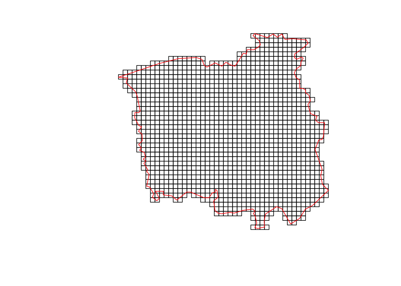
summary(grid)Object of class SpatialPolygonsDataFrame
Coordinates:
min max
x 343.45 366.45
y 410.29 431.79
Is projected: NA
proj4string : [NA]
Data attributes:
layer id Y cellarea
Min. : 0.0000 Min. : 10.0 Min. : 0.0000 Min. :0.25
1st Qu.: 0.0000 1st Qu.: 658.8 1st Qu.: 0.0000 1st Qu.:0.25
Median : 0.0000 Median :1110.5 Median : 0.0000 Median :0.25
Mean : 0.7128 Mean :1072.8 Mean : 0.7128 Mean :0.25
3rd Qu.: 0.0000 3rd Qu.:1485.2 3rd Qu.: 0.0000 3rd Qu.:0.25
Max. :19.0000 Max. :1971.0 Max. :19.0000 Max. :0.25 Now that we have prepared all the data, we can fit the model using R-INLA. To do so, we have to specify a formula and fit the model using the inla() function. For reference, check inla.doc("matern2d").
# Change prior of the precision parameter from (1 / sigma^2) ~ Gamma(1, 0.0005) for PC prior for sigma
# Prob(sigma > u) = alpha
prior.list <- list(prec = list(prior = "pc.prec", param = c(0.25, 0.01))) # c(u, alpha)

formula <- Y ~ 1 + f(id, model = "matern2d", nrow = n_row, ncol = n_col, nu = 1, hyper = prior.list) # Intercept + Matérn spatial random effects

res <- inla(formula,
            family = "poisson",
            data = grid@data,
E = cellarea) # Acts like an offsetsummary(res)
Call:
   c("inla.core(formula = formula, family = family, contrasts = contrasts,
   ", " data = data, quantiles = quantiles, E = E, offset = offset, ", "
   scale = scale, weights = weights, Ntrials = Ntrials, strata = strata,
   ", " lp.scale = lp.scale, link.covariates = link.covariates, verbose =
   verbose, ", " lincomb = lincomb, selection = selection, control.compute
   = control.compute, ", " control.predictor = control.predictor,
   control.family = control.family, ", " control.inla = control.inla,
   control.fixed = control.fixed, ", " control.mode = control.mode,
   control.expert = control.expert, ", " control.hazard = control.hazard,
   control.lincomb = control.lincomb, ", " control.update =
   control.update, control.lp.scale = control.lp.scale, ", "
   control.pardiso = control.pardiso, only.hyperparam = only.hyperparam,
   ", " inla.call = inla.call, inla.arg = inla.arg, num.threads =
   num.threads, ", " keep = keep, working.directory = working.directory,
   silent = silent, ", " inla.mode = inla.mode, safe = FALSE, debug =
   debug, .parent.frame = .parent.frame)" )
Time used:
    Pre = 1.74, Running = 4.91, Post = 0.0908, Total = 6.74
Fixed effects:
              mean    sd 0.025quant 0.5quant 0.975quant   mode kld
(Intercept) -2.106 0.422     -3.013    -2.08     -1.351 -2.018   0

Random effects:
  Name    Model
    id Matern2D model

Model hyperparameters:
                  mean    sd 0.025quant 0.5quant 0.975quant  mode
Precision for id 0.246 0.027      0.195    0.246       0.30 0.247
Range for id     5.792 0.509      4.893    5.757       6.89 5.661

Marginal log-Likelihood:  -1073.43
 is computed
Posterior summaries for the linear predictor and the fitted values are computed
(Posterior marginals needs also 'control.compute=list(return.marginals.predictor=TRUE)')
Now, we can plot the random effects.
grid$R.E. <- res$summary.random$id[grid$id, "mean"]

gridborder <- gUnaryUnion(grid) # Plot the random effects using `tmap` package
tm_shape(grid) +
  tm_polygons(col = c("R.E."), style = "cont", border.col = "transparent", midpoint = NA) +
  tm_shape(gridborder) +
  tm_borders() +
  tm_facets(ncol = 1) +
  tm_legend(legend.position = c("left", "bottom")) + tm_layout(fontfamily = "LM Roman 10", frame = FALSE)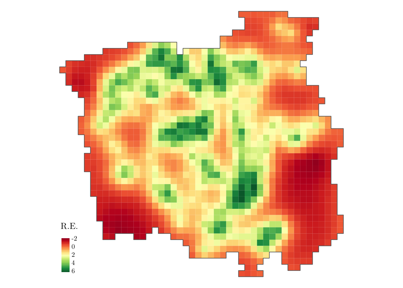
From the above map, we observe a non-constant pattern of the spatially structured random effect suggesting that the intensity of the process that generates the cancer-diagnosed patients’ locations may be affected by other spatial factors that have not been considered in the model.
cellarea   <- resolution * resolution
grid$Mean  <- res$summary.fitted.values[, "mean"] * cellarea
grid$Lower <- res$summary.fitted.values[, "0.025quant"] * cellarea
grid$Upper <- res$summary.fitted.values[, "0.975quant"] * cellarea

# Changing the margin size to accommodate the plot caption
bbox_new <- st_bbox(grid)
xrange <- bbox_new$xmax - bbox_new$xmin # range of x values
yrange <- bbox_new$ymax - bbox_new$ymin # range of y values

bbox_new[1] <- bbox_new[1] - (0.25 * xrange)
bbox_new    <- bbox_new %>% st_as_sfc()

# Main plot for the estimated intensity (along with a 95% equal-tail credible interval)
tm_shape(grid, bbox = bbox_new) +
  tm_polygons(col = c("Lower", "Mean", "Upper"),
              style = 'fixed', border.col = "transparent",
              breaks = c(0, 0.25, 0.5, 0.75, 1.0, 2, 5, 10, ceiling(max(grid$Upper)) + 1)) +
  tm_shape(gridborder) +
  tm_borders() +
  tm_facets(nrow = 3) +
  tm_legend(legend.position = c("left", "bottom")) +
  tm_layout(fontfamily = "LM Roman 10", frame = FALSE, inner.margins  = c(0, 0, 0, 0))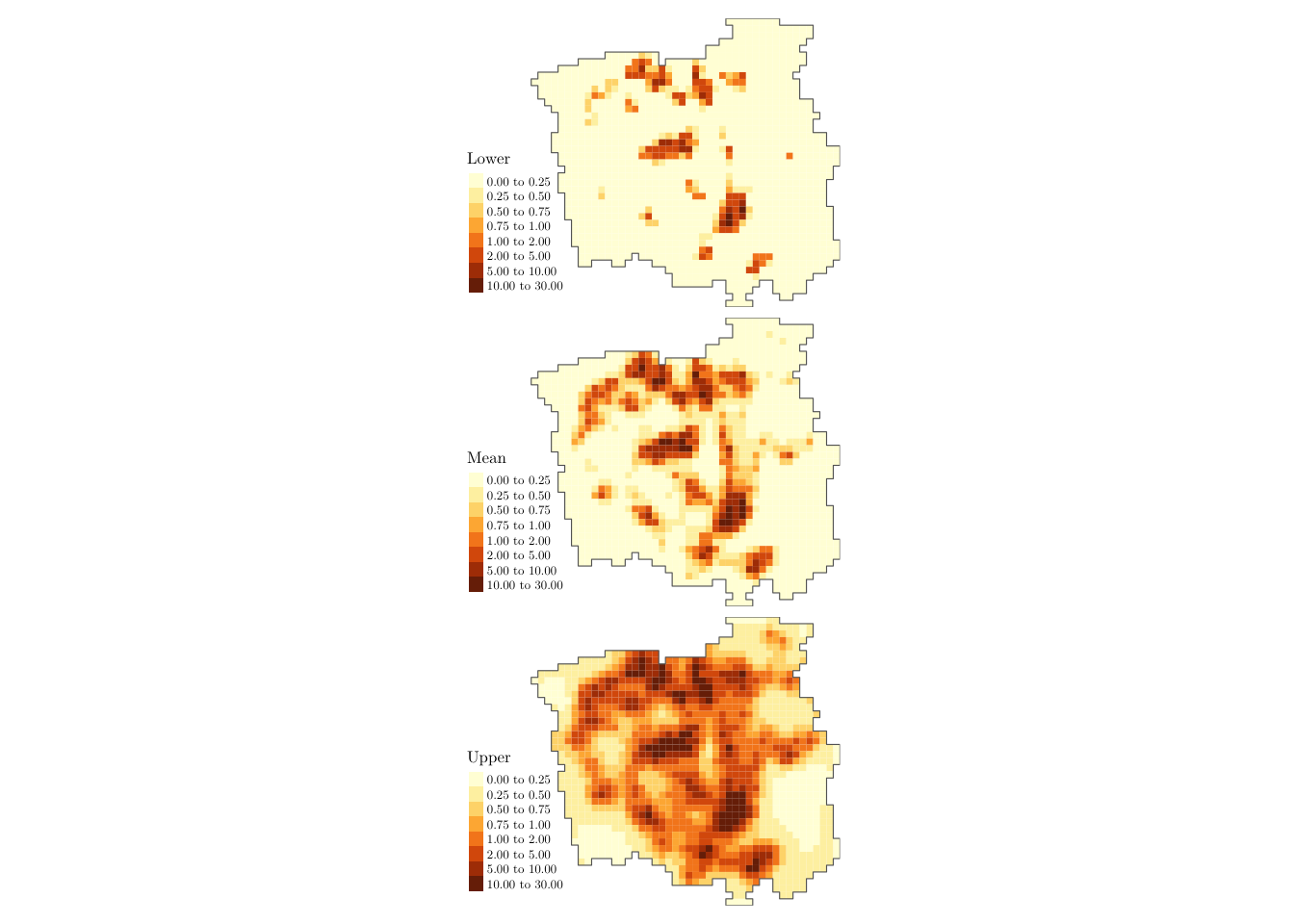
From the above plot, we can identify (while also accounting for the estimating uncertainty) the areas with high incidence of lung-cancer patients (denoted by the estimated intensity process). Based on such information, policymakers can focus their resources on regions that matter the most when dealing with cancer management.
We can also include a temporal random effect in the R-INLA formula (e.g., f(id_time, model = "ar1")), with possibly space-time interaction terms (Held, 2000). That is precisely what we will do in our next example.
Example 2
For this example, we will analyze the location of terrorism attacks in a given country over the years. The two data objects (terror_country.rds and area_country.rds) can be downloaded from here and here, respectively.
terror_country <- readRDS(file = "terror_country.rds")
table(terror_country$country)
  AFG   AGO   ALB   ARE   ARG   ARM   AUS   AUT   AZE   BDI   BEL   BFA   BGD
 4783     1     6     4    13     5    33     5     4   204     9    17   813
  BGR   BIH   BLR   BRA   CAF   CAN   CHE   CHL   CHN   CIV   CMR   COD   COG
   11     9     6    10   112    22     5    40    54    31   118   353     2
  COL   CYP   CZE   DEU   DOM   DZA   ECU   EGY   ERI   ESP   EST   ETH   FIN
  659    13    14   126     1   169     6   550    16    17     3    31    10
  FRA   GBR   GEO   GHA   GIN   GNB   GRC   GTM   GUY   HND   HRV   HTI   HUN
  106   330    20     2     4     2   217     4     1     4     5     1     3
  IDN   IND   IRL   IRN   IRQ   ISL   ISR   ITA   JAM   JOR   JPN   KAZ   KEN
  125  4190   133    61 15022     2   324    49     1    14    16    16   279
  KGZ   KHM   KOR   KWT   LAO   LBN   LBR   LBY   LKA   MAR   MDA   MDG   MEX
   10     2     2     3     2   219     2  1156    19     2     2     6    48
  MKD   MLI   MMR   MNE   MOZ   MRT   MWI   MYS   NER   NGA   NIC   NLD   NOR
    7   278   108     3    88     2     1    36    86  2458     1    12     4
  NPL   NZL   PAK   PAN   PER   PHL   POL   PRT   PRY   PSE   QAT   RUS   RWA
  224     2  8116     1    22  2328     2     2    49   527     1   707    26
  SAU   SDN   SEN   SLE   SOM   SSD   SVK   SWE   SWZ   SYR   TCD   THA   TJK
  153   381    10     1  2087   120     1    52     1  1398    26  1039     8
  TKM   TTO   TUN   TUR   TWN   TZA   UGA   UKR   URY   USA   UZB   VEN   YEM
    7     3    61   651     2    19    32  1373     1   188     1    14  1712
  YUG   ZAF   ZWE
   28    61     5
Aiming to have a larger data set, we analyze the country with the highest number of observed events, i.e., IRQ. Also, we will analyze observed events that occurred from 2010 to 2015.
country_code <- "IRQ"

terror_country <- terror_country[terror_country$country == country_code, ]
terror_country <- terror_country[(terror_country$iyear >= 2010) & (terror_country$iyear <= 2015), ]
coordinates(terror_country) <- c("longitude", "latitude")
proj4string(terror_country) <- "+proj=longlat"

area_country <- readRDS(file = "area_country.rds")
area_country <- area_country[area_country$sov_a3 == country_code, ]
area_country <- spTransform(x = area_country, CRSobj = CRS("+proj=longlat"))

plot(area_country, main = "")
plot(terror_country, add = T, col = "green")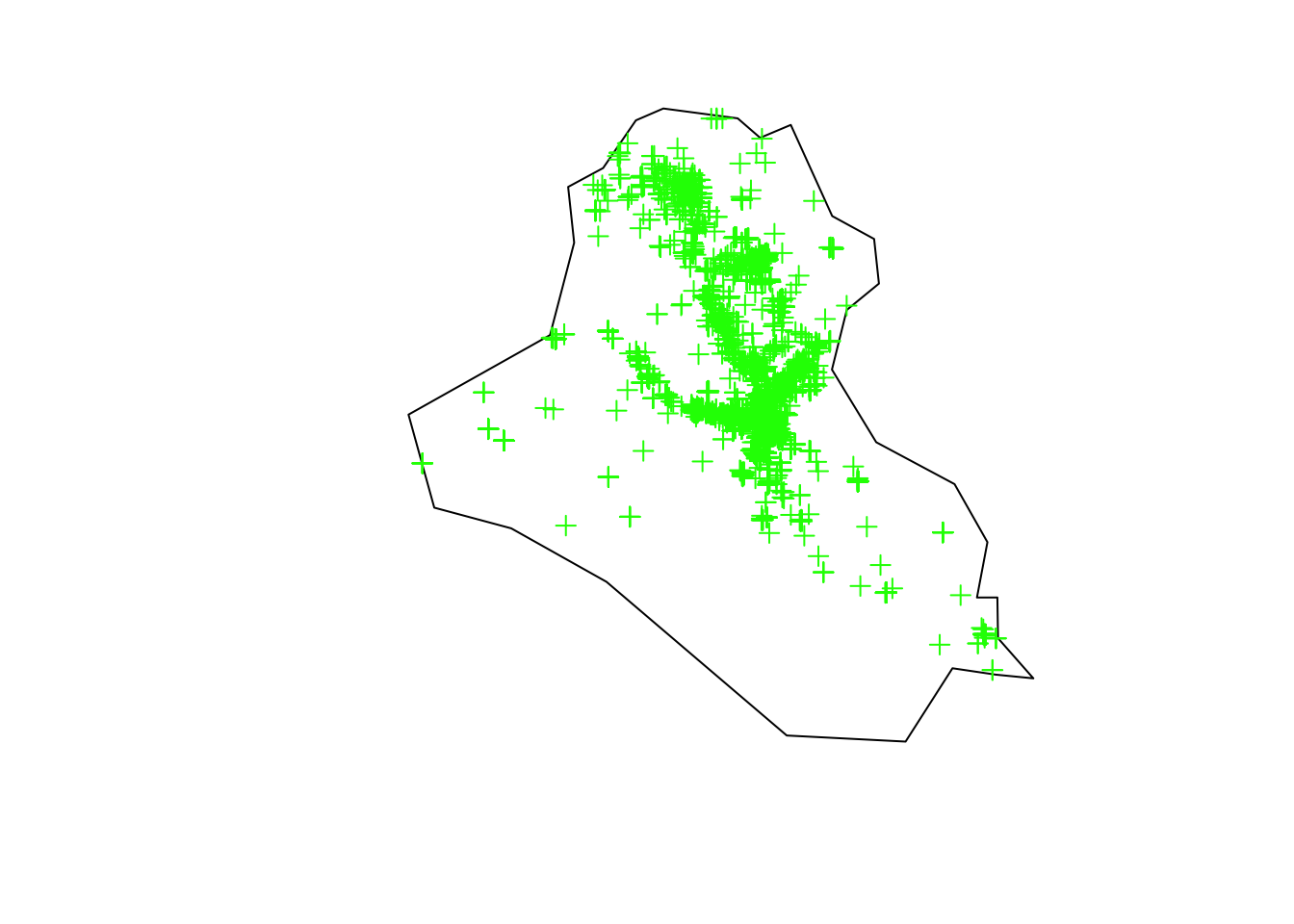
Now, given a partition, we can do as before, and count the number of events in each cell. However, notice that we also have to account for the variable year when doing so.
resolution <- 0.5
r <- raster(area_country, resolution = resolution)
(n_row <- nrow(r))
[1] 17(n_col <- ncol(r))[1] 20terror_country$year <- terror_country$iyear - min(terror_country$iyear) + 1
n_years <- length(unique(terror_country$year))
tab <- list()
ras <- list()
grids <- list()
grids_map <- list()
par(mfrow = c(2, 3), mar = c(2, 2, 2, 6) + 1)
for (y in 1:n_years) {
tab[[y]] <- table(cellFromXY(r, terror_country[terror_country$year == y, ]))
ras[[y]] <- r
ras[[y]][as.numeric(names(tab[[y]]))] <- tab[[y]]
values(ras[[y]])[is.na(values(ras[[y]]))] <- 0
grids[[y]] <- rasterToPolygons(ras[[y]])
grids[[y]] <- grids[[y]][as.vector(matrix(1:nrow(grids[[y]]), nrow = n_row, ncol = n_col, byrow = T)), ]
grids[[y]]$id <- 1:nrow(grids[[y]])
grids[[y]]$Y <- grids[[y]]$layer
grids[[y]]$cellarea <- resolution * resolution
grids_map[[y]] <- raster::intersect(x = grids[[y]], y = area_country)
grids[[y]] <- grids[[y]][grids[[y]]$id %in% grids_map[[y]]$id, ]
plot(ras[[y]], main = y)
plot(area_country, add = T)
}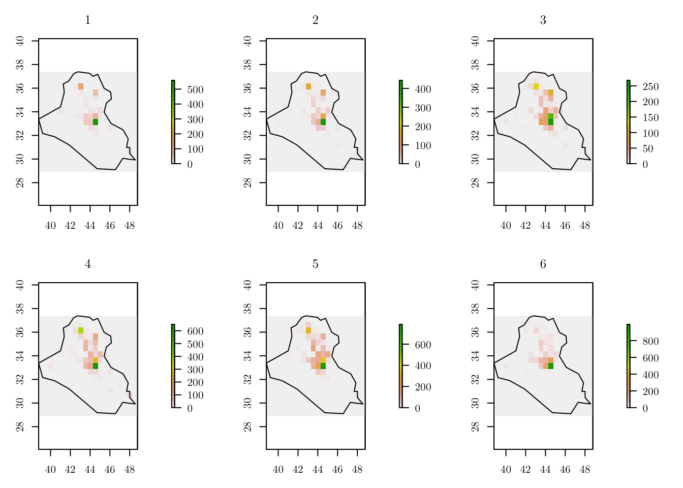
par(mfrow = c(1, 1))Then, we can create a data object with the extra id_time index.
for (y in 1:n_years) {
  if (y == 1) {
    data_inla <- grids[[y]]@data
  } else {
    data_inla <- rbind(data_inla, grids[[y]]@data)
  }
}
data_inla <- cbind(data_inla, id_time = rep(x = 1:n_years, each = nrow(grids[[1]])))
data_inla[c(1:3, ((nrow(data_inla) - 2):nrow(data_inla))), ]
layer id Y cellarea id_time
141 0 8 0 0.25 1
161 0 9 0 0.25 1
181 0 10 0 0.25 1
2795 2 320 2 0.25 6
2995 1 321 1 0.25 6
3005 0 338 0 0.25 6Finally, we can fit the model. In our case, we will define \begin{align*} \zeta(x, t) = \zeta_1(x) + \zeta_2(t), \end{align*} where \zeta_1(x) is a spatial model (e.g., Matérn) and \zeta_2(t) is a temporal model (e.g., AR1).
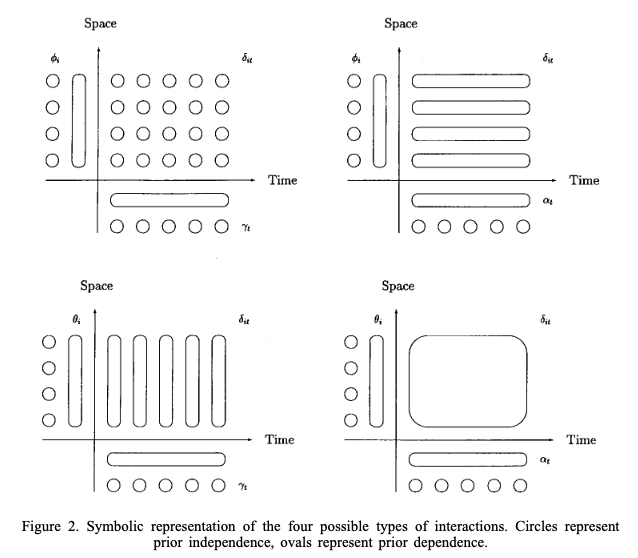
Alternatively, we could fit a model with interaction. For example, for x_i \in \mathcal{D}, \begin{align*} \zeta(x_i, t) = \alpha \zeta(x_i, t - 1) + \phi(x_i, t) \end{align*} where |\alpha| < 1 and \zeta(x, 1) follows a stationary distribution of a first-order autoregressive process (AR1), namely \text{Normal}(0, \sigma^2_{\omega}/(1 - \alpha^2)). And each \phi(x, t) follows a zero-mean Gaussian distribution temporally independent but spatially dependent at each time. In general, from Held, 2000,
Getting back to the chosen model, we have
prior.list <- list(prec = list(prior = "pc.prec", param = c(0.25, 0.01))) # Priors

# Separable space-temporal model: eta_ij = beta_0 + u_i + v_j
formula <- Y ~ 1 + f(id,
                     model = "matern2d",
                     nrow = n_row,
                     ncol = n_col,
                     nu = 1,
                     hyper = prior.list) + f(id_time, model = "ar1")

# Model with interaction: eta_ij = beta_0 + u_ij
# formula <- Y ~ 1 + f(id,
#                      model = "matern2d",
#                      nrow = n_row,
#                      ncol = n_col,
#                      nu = 1,
#                      group = id_time,
#                      control.group = list(model = "ar1"),
#                      hyper = prior.list)

res <- inla(formula,
            family = "poisson",
            data = data_inla,
E = resolution)summary(res)
Call:
c("inla.core(formula = formula, family = family, contrasts = contrasts,
", " data = data, quantiles = quantiles, E = E, offset = offset, ", "
scale = scale, weights = weights, Ntrials = Ntrials, strata = strata,
", " lp.scale = lp.scale, link.covariates = link.covariates, verbose =
verbose, ", " lincomb = lincomb, selection = selection, control.compute
= control.compute, ", " control.predictor = control.predictor,
control.family = control.family, ", " control.inla = control.inla,
control.fixed = control.fixed, ", " control.mode = control.mode,
control.expert = control.expert, ", " control.hazard = control.hazard,
control.lincomb = control.lincomb, ", " control.update =
control.update, control.lp.scale = control.lp.scale, ", "
control.pardiso = control.pardiso, only.hyperparam = only.hyperparam,
", " inla.call = inla.call, inla.arg = inla.arg, num.threads =
num.threads, ", " keep = keep, working.directory = working.directory,
silent = silent, ", " inla.mode = inla.mode, safe = FALSE, debug =
debug, .parent.frame = .parent.frame)" )
Time used:
Pre = 2.12, Running = 1.76, Post = 0.062, Total = 3.94
Fixed effects:
mean sd 0.025quant 0.5quant 0.975quant mode kld
(Intercept) -2.786 0.611 -4.033 -2.769 -1.63 -2.768 0
Random effects:
Name Model
id Matern2D model
id_time AR1 model
Model hyperparameters:
mean sd 0.025quant 0.5quant 0.975quant mode
Precision for id 0.164 0.021 0.125 0.164 0.208 0.164
Range for id 2.836 0.288 2.317 2.819 3.452 2.782
Precision for id_time 8.147 2.760 4.044 7.712 14.776 6.911
Rho for id_time 0.569 0.102 0.341 0.579 0.739 0.603
Marginal log-Likelihood: -2303.43
is computed
Posterior summaries for the linear predictor and the fitted values are computed
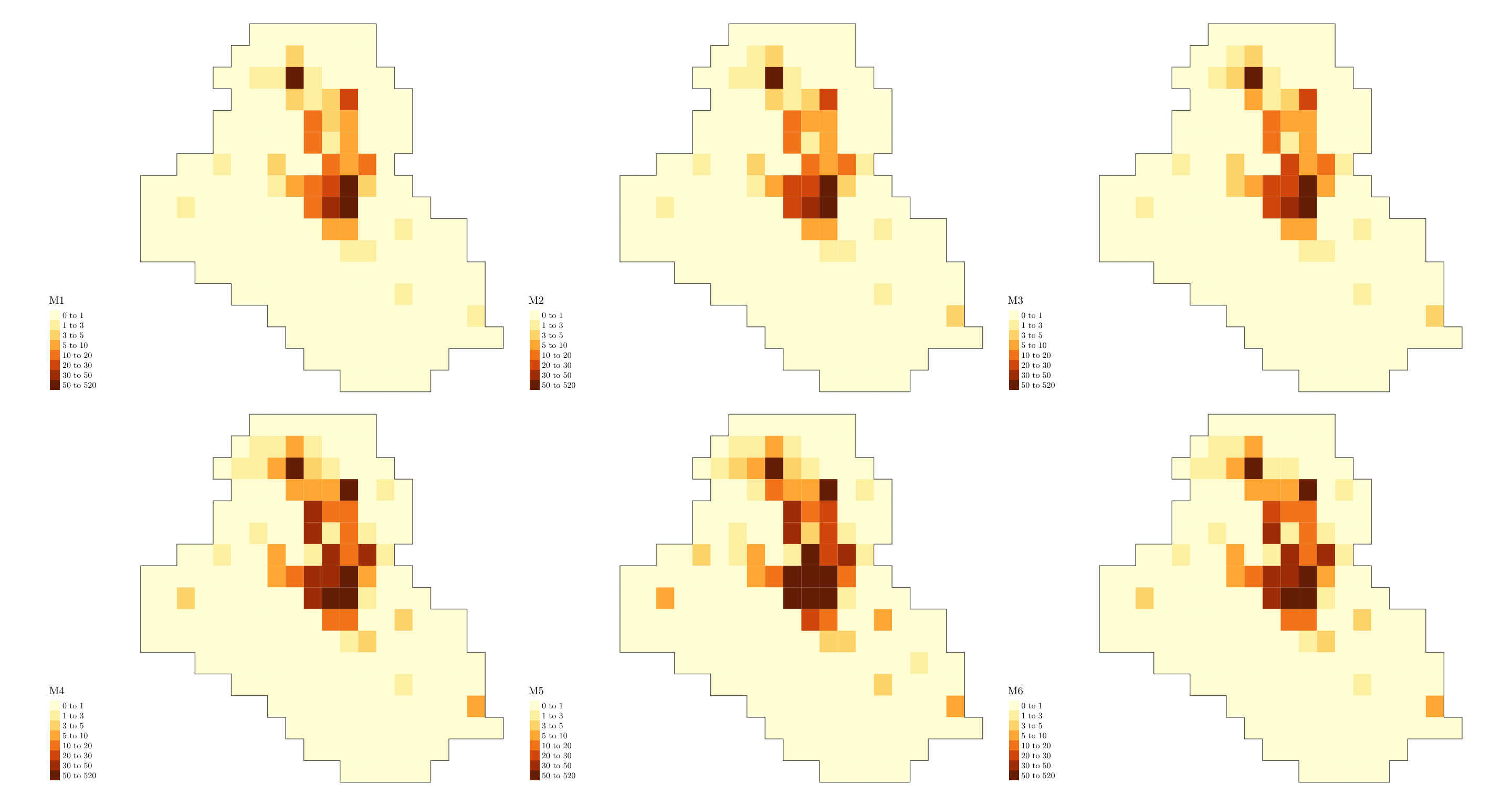
(Posterior marginals needs also 'control.compute=list(return.marginals.predictor=TRUE)')astly, as in the previous example, we can plot the estimated intensity for all years.
grid       <- grids[[1]]
cells_grid <- nrow(grids[[1]])
cellarea   <- resolution * resolution

grid$M1 <- res$summary.fitted.values[, "mean"][1:cells_grid] * cellarea
grid$M2 <- res$summary.fitted.values[, "mean"][(cells_grid + 1):(cells_grid * 2)] * cellarea
grid$M3 <- res$summary.fitted.values[, "mean"][(cells_grid * 2 + 1):(cells_grid * 3)] * cellarea
grid$M4 <- res$summary.fitted.values[, "mean"][(cells_grid * 3 + 1):(cells_grid * 4)] * cellarea
grid$M5 <- res$summary.fitted.values[, "mean"][(cells_grid * 4 + 1):(cells_grid * 5)] * cellarea
grid$M6 <- res$summary.fitted.values[, "mean"][(cells_grid * 5 + 1):(cells_grid * 6)] * cellarea

max_int <- ceiling(max(c(grid$M1, grid$M2, grid$M3, grid$M4, grid$M5, grid$M6)))
max_int <- ceiling(max_int / 10) * 10

bbox_new <- st_bbox(grid)
xrange <- bbox_new$xmax - bbox_new$xmin # range of x values
yrange <- bbox_new$ymax - bbox_new$ymin # range of y values

bbox_new[1] <- bbox_new[1] - (0.25 * xrange)
bbox_new <- bbox_new %>% st_as_sfc()

gridborder <- gUnaryUnion(grid)
tm_shape(grid, bbox = bbox_new) +
  tm_polygons(col = c("M1", "M2", "M3", "M4", "M5", "M6"),
              style = 'fixed', border.col = "transparent",
              breaks = c(0, 1, 3, 5, 10, 20, 30, 50, max_int)) +
  tm_shape(gridborder) + tm_borders() +
  tm_facets(ncol = 3) + tm_legend(legend.position = c("left", "bottom")) +
  tm_layout(fontfamily = "LM Roman 10", frame = FALSE)