Survival Models (MATH3085/6143)

Chapter 1-9: Survival Models

André Victor Ribeiro Amaral

a.v.ribeiro-amaral@soton.ac.uk

University of Southampton

12/11/2025

Chapter 1: Introduction

• Survival analysis refers to a set of special statistical methods required to analyse time-to-event \(T\).

• Why is Survival Analysis “special”?
  • Models for non-negative random variable \(T\).
  • Data are typically censored.

Chapter 1: Introduction (vevox.app, 129-515-844)

1. Which type of censoring occurs when an observation ends before the event of interest has been observed?

1. Left censoring
2. Right censoring
3. Interval censoring
4. This is an example of truncation

2. Which of the following is an example of non-informative censoring?

1. A patient leaves the study because their health is rapidly improving
2. An experimental machine is removed from the trial because it developed a new, unrecorded fault
3. The study concludes on the final pre-scheduled date, and the subject is still alive
4. A subject withdraws from a drug trial after experiencing severe side effects

Chapter 2: Statistical Models

Parametric statistical model: for the leukaemia survival times, a common model would be \[ T_1,T_2,\cdots , T_n \stackrel{\text{i.i.d.}}{\sim} \mathrm{lognormal}(\mu,\sigma^2) \] where \(\mu\) and \(\sigma^2\) are unspecified.

Non-parametric statistical model: sometimes, it is not appropriate, or we want to avoid, making a precise specification for the distribution which generated \(T_1,T_2,\cdots , T_n\).

Then, we might propose the model \[ T_1,T_2,\cdots , T_n \text{ are i.i.d. random variables.} \]

Regression model: we model survival data to learn about the relationship between survival time \(T\) and other potentially explanatory variables \(x_1, x_2, \cdots\).

Chapter 3: The Survival distribution

• If \(T\) is a continuous random variable, then its distribution is defined by its probability density function \(f_T(t)\), or \(f(t)\) for short.

• The distribution function \(F_T(t)\), for a random variable \(T\), is defined as \(F_T(t)=\mathbb{P}(T\le t)\).

• The survival function \(S_T(t)\), for a random variable \(T\), is defined as \(S_T(t)=\mathbb{P}(T > t)\).

• The hazard function \(h_T(t)\) is defined, for \(t \geq 0\), as \[ h_T(t) = \lim_{\delta t\to 0}\frac{\mathbb{P}(T\le t+\delta t|T> t)}{\delta t}. \]

• The cumulative hazard function \(H_T(t)\) is defined as \(H_T(t)=\int_0^t h_T(u) du\).

Chapter 3: The Survival distribution

• Only one of the functions \(f_T\), \(F_T\), \(S_T\), \(h_T\), or \(H_T\) needs to be specified to completely determine the distribution of \(T\).

Relationships

	\[f_T\]	\[S_T\]	\[h_T\]
\[f_T(t) = \]		\[-\frac{\mathrm{d}}{\mathrm{d}t} S_T(t)\]	\[h_T(t)\exp\left[-\int_0^t h_T(s)\mathrm{d}s\right]\]
\[S_T(t) = \]	\[\int_t^\infty f_T(s)\mathrm{d}s\]		\[\exp\left[-\int_0^t h_T(s)\mathrm{d}s\right]\]
\[h_T(t) = \]	\[\frac{f_T(t)}{\int_t^\infty f_T(s)\mathrm{d}s}\]	\[-\frac{\mathrm{d}}{\mathrm{d}t} \log S_T(t)\]

Chapter 3: The Survival distribution (vevox.app, 129-515-844)

3. The expected lifetime \(\mathbb{E}(T)\) is given by

1. The integral of \(f_T(t) / S_T(t)\) over \([0, t]\)
2. The slope of the survival function
3. The integral of the survival function, \(S_T(t)\), from \(0\) to \(\infty\).
4. The integral of PDF, \(f_T(t)\), from \(0\) to \(t\).

4. How is the hazard function \(h_T(t)\) related to the PDF and survival function?

1. \(h_T(t) = f_T(t) \cdot S_T(t)\)
2. \(h_T(t) = -\frac{d}{dt} f_T(t)\)
3. \(h_T(t) = f_T(t) / S_T(t)\)
4. \(h_T(t) = S_T(t) / f_T(t)\)

Chapter 4: Distributions for Survival Models

We introduced some common distributions when working with time-to-event data, namely

• \(\text{Exponential}(\beta)\): constant hazard.

• \(\text{Weibull}(\alpha, \beta)\): generalises the Exponential model; \(\text{Weibull}(\alpha = 1, \beta) \equiv \text{Exponential}(\beta)\).

• \(\text{Log-logistic}(\alpha, \beta)\): non-monotonic hazard.

• \(\text{Log-normal}(\mu, \sigma^2)\): non-monotonic hazard (different rate of decay).

• \(\text{Gompertz}(\alpha, \beta)\): risk of death increases exponentially (used to model human lifetime from middle age onwards).

• \(\text{Makeham}(\alpha, \beta, \lambda)\): generalises the Gompertz model.

Chapter 4: Distributions for Survival Models (vevox.app, 129-515-844)

5. If \(X \sim \text{Exp}(1)\), which transformation \(T = g(X)\) yields a Weibull distribution, i.e., \(T \sim \text{Weibull}(\alpha, \beta)\)?

1. \(T = X / \beta\)
2. \(T = \exp\left\{\frac{X}{\beta}\right\}\)
3. \(T = \left(\frac{X}{\beta}\right)^{1/\alpha}\)
4. \(T = \frac{X^{1/ \alpha}}{\beta}\)

Chapter 5: Survival models: parameter estimation

• In a parametric model, estimating the distribution of \(T\) simply involves estimating the unknown parameters \(\theta\).

• Typically, we use maximum likelihood estimation to obtain \(\hat{\boldsymbol{\theta}}\).

• Assuming iid observations with (right) censoring indicators \(d_1,\cdots ,d_n\), the likelihood function is \[ L(\theta)=\prod_{i:d_i=1} f_T(t_i;\theta)\prod_{i:d_i=0} S_T(t_i;\theta) \]

• For large samples, we have the asymptotic approximation \[ \hat{\theta}\;\;\stackrel{\text{approx.}}{\sim}\; \text{Normal}(\theta, I(\theta)^{-1}). \]

Chapter 5: Survival models: parameter estimation (vevox.app, 129-515-844)

6. In the likelihood function \(L(\theta)\) for a single right-censored observation \(t_i\) (\(d_i=0\)), what is the appropriate contribution?

1. The survival function \(S_T(t_i; \theta)\)
2. The hazard function \(h_T(t_i; \theta)\)
3. The distribution function \(F_T(t_i; \theta)\)
4. The PDF \(f_T(t_i; \theta)\)

7. The standard error \(\text{se}(\hat{\theta})\) for the maximum likelihood estimator \(\hat{\theta}\) is computed in the following way

1. \(I(\hat{\theta})^{-1}\)
2. \(\sqrt{I(\hat{\theta})^{-1}}\)
3. \(I(\hat{\theta})\)
4. \(\sqrt{I(\hat{\theta})}\)

Chapter 6: Non-parametric Survival Estimation

Recall that the likelihood is given by

\[ L(\theta)=\prod_{i:d_i=1} f_T(t_i; \theta)\prod_{i:d_i=0} S_T(t_i; \theta). \]

Without assuming a particular parametric family for \(f_T\), the likelihood \(L(\theta)\) can be made infinitely large.

To resolve this, the non-parametric maximum likelihood estimate of the survival distribution is taken to be a discrete distribution supported on the observed failure times \(\{t_i: d_i=1\}\).

The discrete hazard MLE is \[ \hat{h}_i=\frac{d'_i}{r_i},\qquad i=1,\cdots, m, \qquad \text{ where } \qquad r_i=\sum_{j=i}^m (d'_j+c_j) \] is the number at risk at \(t'_i\) \((\text{failures} + \text{censored observations})\).

Chapter 6: Non-parametric Survival Estimation

The corresponding estimator of the survival function \[ \hat{S}(t)=\prod_{j=1}^i (1-\hat{h}_j)=\prod_{j=1}^i \left(1-\frac{d'_j}{r_j}\right)\qquad t\in[t'_i,t'_{i+1}), \quad i=0,\cdots ,m \] is called the Kaplan-Meier (or product-limit) estimator.

Consider the following survival times \(\mathbf{t} = \left(3, 4, 6^*, 8, 8, 10\right)\) (i.e., \(m=4\) distinct observations).

\(i\)	\(t_i\)	\(t_{i+1}\)	\(r_i\)	\(d_i'\)	\(c_i\)	\(\hat{S}(t)\)
\(0\)	\(0\)	\(3\)	\(6\)	\(0\)	\(0\)	\(1\)
\(1\)	\(3\)	\(4\)	\(6\)	\(1\)	\(0\)	\(\frac{5}{6}\)
\(2\)	\(4\)	\(8\)	\(5\)	\(1\)	\(1\)	\(\frac{2}{3}\)
\(3\)	\(8\)	\(10\)	\(3\)	\(2\)	\(0\)	\(\frac{2}{9}\)
\(4\)	\(10\)	\(\infty\)	\(1\)	\(1\)	\(0\)	\(0\)

par(family = "Latin Modern Roman 10", mar = c(5.1, 4.1, 0.5, 2.1))
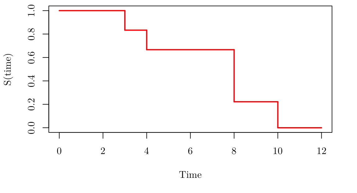
plot(0, 0, type="l", xlim=c(0,12), ylim=c(0,1), xlab = "Time", ylab = "S(time)")
segments(x0 = c(0, 3, 4, 8, 10), x1=c(3, 4, 8, 10, 12), y0=c(1, 5/6, 2/3, 2/9,0), y1 = c(1, 5/6, 2/3, 2/9, 0), lwd = 2, col = "red")
segments(x0 = c(3, 4, 8, 10),    x1=c(3, 4, 8, 10),     y0=c(1, 5/6, 2/3, 2/9  ), y1 = c(5/6, 2/3, 2/9, 0   ), lwd = 2, col = "red")

Chapter 6: Non-parametric Survival Estimation (vevox.app, 129-515-844)

8. When times are tied (e.g., a failure and a censoring occur at \(t^*\)), the KM convention treats the censored time as

1. Being removed entirely from the analysis
2. Infinitesimally smaller than the failure time
3. A full failure event (\(d_i=1\))
4. Infinitesimally larger than the failure time

Chapter 7: Survival Regression Models

A proportional hazards model (or Cox regression model) assumes that the hazard function for the survival variable corresponding to the \(i\)-th unit is \[ h_{T_i}(t)=\exp\left\{\mathbf{x}_i^{\top}\boldsymbol{\beta}\right\}\cdot h_0(t) \] where \(h_0\) is called the baseline hazard function and is not assumed to have a particular mathematical form.

The partial likelihood is given by \[ \begin{eqnarray*} L(\boldsymbol{\beta}) = \prod_{i:d_i=1}\frac {\exp\left(\mathbf{x}_i^{\top}\boldsymbol{\beta}\right)} {\sum_{j\in R_i} \exp\left(\mathbf{x}_j^{\top}\boldsymbol{\beta}\right)}. \end{eqnarray*} \]

An accelerated failure time (AFT) model is generally expressed through the survival function \[ S_{T_i}(t)=S_0\left(t \cdot \exp (-\eta_i)\right) \] for some parametric baseline survival function \(S_0\).

Chapter 7: Survival Regression Models (vevox.app, 129-515-844)

9. In the Partial Likelihood denominator, the sum \(\sum_{j \in R_i} \exp(\mathbf{x}_j^{\top}\boldsymbol{\beta})\) represents the

1. Total likelihood of the uncensored observations
2. Number of failures observed at time \(t_i\)
3. Baseline hazard function \(h_0(t)\)
4. Total expected risk (hazard) across all individuals in the risk set \(R_i\).

10. If the estimated coefficient \(\hat{\beta}\) in a Cox model is negative \((\text{i.e., }\exp(\hat{\beta}) < 1)\), what does this imply about the covariate’s effect?

1. The covariate decreases the hazard rate (better survival)
2. The hazard function is non-monotonic
3. The baseline hazard \(h_0(t)\) is zero
4. The covariate increases the hazard rate

Chapter 8: Multistate Survival Models

Alternatively, one can model the variable \(Y_t\) representing the status (alive or dead) of a unit at time \(t\).

The transition probabilities are defined as \(\mathbb{P}(Y_{x+t}=j\,|\,Y_x=i)\;\equiv\;p_{ij}(x,t), ~~ j\in S.\)

The transition intensity function \(\mu_{ij}(x)\) is defined as \(\mu_{ij}(x)=\lim_{\delta t\to 0} \frac{p_{ij}(x,\delta t)}{\delta t}, ~~ i\ne j.\)

How are the transition probabilities \(p_{ij}(x,t)\) obtained from the transition intensities \(\mu_{ij}(x)\)?

The Kolmogorov forward equations: \(\frac{d}{dt} p_{ij}(x,t) = \sum_{k\in S} p_{ik}(x,t) \cdot \mu_{kj}(x+t), ~~ i,j\in S\).

Chapter 8: Multistate Survival Models (vevox.app, 129-515-844)

11. In a time-homogeneous Markov process, the transition intensities \(\mu_{ij}(x)\), \(i \neq j\), are

1. Always equal to \(1\)
2. Dependent on the entire prior history of the process
3. Dependent on the current state \(i\), but not dependent on the current time \(x\)
4. Always zero for all states \(i\) and \(j\)

12. For a time-homogeneous Markov process, the holding time distribution \(T_{xi}\) is always what type of distribution?

1. Weibull
2. Normal
3. Log-logistic
4. Exponential

Chapter 9: Inference for Multistate Models

For \(n = 1\), we might observe something like

Transition	Start	1	2	3	4	5	6	7	8	9	10	11	End
Time	0.3	0.32	0.41	0.56	0.82	0.84	1.31	1.41	1.55	1.79	2.04	2.24	2.80
State	2	1	3	4	1	2	1	3	2	3	1	2	2

The likelihood for the full set of transition intensity parameters \(\boldsymbol{\mu}=\{\mu_{k\ell},k\ne\ell\}\) for a single individual transition history is

\[ \begin{eqnarray*} L(\boldsymbol{\mu})&=&S_{y_{J}}(t_{J+1}-t_{J}) \prod_{j=1}^J f_{y_{j-1}}(t_{j}-t_{j-1})p(y_j|y_{j-1})\\ &=& \prod_{k,\ell:k\ne \ell}\mu_{k\ell}^{n_{k\ell}} \cdot \exp\left(-t^+_k \mu_{k\ell}\right), \end{eqnarray*} \]

• \(t^+_k\) is the total observed holding time in state \(k\)
• \(n_{k\ell}\) is the total observed number of transitions from state \(k\) to state \(\ell\)

Chapter 9: Inference for Multistate Models (vevox.app, 129-515-844)

13. If the likelihood \(L(\boldsymbol{\mu})\) is calculated for multiple individuals \((n > 1)\), how is the joint likelihood obtained?

1. By averaging the individual log-likelihoods
2. By multiplying the individual likelihoods, assuming independence
3. By using numerical methods only
4. By summing the individual likelihoods