Survival Models (MATH3085/6143)

Chapter 7: Survival Regression Models

André Victor Ribeiro Amaral

a.v.ribeiro-amaral@soton.ac.uk

University of Southampton

22/10/2025

Recap

In the last chapter, we

• Defined the non-parametric MLE: we resolved the problem of the unbounded likelihood by constructing a the Non-Parametric Maximum Likelihood Estimator of the survival distribution based on a discrete distribution with mass only at the observed failure times.

• Derived the Kaplan-Meier estimator for the survival function \(\hat{S}(t)\).

• Learned how to calculate the variance using Greenwood’s formula and how to use the Nelson-Aalen estimator \(\hat{H}(t)\) and its resulting Fleming-Harrington survival curve as alternatives to Kaplan-Meier.

Chapter 7: Survival Regression Models

Introduction

Commonly, when we observe (possibly censored) survival times \(t_1, \cdots ,t_n\), we also observe the values of \(k\) other variables, \(x_1, \cdots ,x_k\), for each of the \(n\) units of observation.

Then, we drop the assumption that the survival time variables \(T_1, \cdots ,T_n\) are identically distributed, and investigate how their distribution depends on the explanatory variables (or covariates) \(x_1, \cdots, x_k\).

In a regression model, we assume that the dependence of the distribution of \(T_i\) on the values of \(x_1, \cdots, x_k\) is through a regression function, which is typically assumed to have linear structure, as \[ \eta_i=\beta_1 x_{i1}+\beta_2 x_{i2}+ \cdots +\beta_k x_{ik}=\sum_{j=1}^k x_{ij}\beta_j=\mathbf{x}_i^{\top}\boldsymbol{\beta} \] where \(\mathbf{x}_i=(x_{i1},x_{i2},\ldots ,x_{ik})^{\top}\) is the \(k\)-vector containing the values of \(x_1,\cdots,x_k\) for unit \(i\) and \(\boldsymbol{\beta}=(\beta_{1},\beta_{2},\ldots ,\beta_{k})^{\top}\) is a \(k\)-vector of regression parameters.

Example: Leukaemia (as in Chapter 2)

Survival times are given for 33 patients who died from acute myelogenous leukaemia. In R, this can be found in the leuk object in the MASS package.

as_tibble(leuk)

# A tibble: 33 × 3
     wbc ag       time
   <int> <fct>   <int>
 1  2300 present    65
 2   750 present   156
 3  4300 present   100
 4  2600 present   134
 5  6000 present    16
 6 10500 present   108
 7 10000 present   121
 8 17000 present     4
 9  5400 present    39
10  7000 present   143
# ℹ 23 more rows

leuk is a data frame with columns: wbc (white blood count), ag (a test result, “present” or “absent”), and time (survival time in weeks).

Example: Leukaemia (as in Chapter 2)

Here, we have two potential explanatory variables, wbc and ag. As ag is a factor (a non-numerical variable) we transform it in the regression function to an indicator (dummy) variable or variables, for example \[ 1(\texttt{ag}~~\text{is present}) = \left\{ \begin{array}{ll} 1 & \text{if}~~\texttt{ag}~~\text{is present}\\ 0 & \text{if}~~\texttt{ag}~~\text{is absent} \end{array} \right. \]

Similarly further explanatory variables may be created from the numeric covariate wbc, e.g. \(\texttt{wbc}^2\) to investigate possible quadratic dependence.

Proportional hazards (Gap on page 59)

As was the case with homogeneous survival models in Chapter 6, we frequently want to investigate the dependence of \(T_i\) on \(x_1, \cdots, x_k\), without assuming a particular parametric family for \(f_{T_i}\).

A proportional hazards model (or Cox regression model) assumes that the hazard function for the survival variable corresponding to the \(i\)-th unit is \[ h_{T_i}(t)=\exp\left\{\mathbf{x}_i^{\top}\boldsymbol{\beta}\right\}\cdot h_0(t) \] where \(h_0\) is called the baseline hazard function and is not assumed to have a particular mathematical form.

Hence, we model the effect of the explanatory variables on the distribution of \(T_i\) as multiplying the baseline hazard by the exponentiated regression function, \(\exp\{\eta_i\}\).

Proportional hazards (Gap on page 60)

Equivalently, \[ \begin{eqnarray*} S_{T_i}(t) & = & \exp\left[ - \int_0^t h_{T_i}(s) \mathrm{d}s \right]\\ & = & \exp\left[ - \int_0^t \exp\left(\mathbf{x}_i^T\boldsymbol{\beta}\right) \cdot h_0(s)\mathrm{d}s \right]\\ & = & \exp\left[ - \int_0^t h_0(s)\mathrm{d}s \right]^{\exp\left(\mathbf{x}_i^{\top}\boldsymbol{\beta}\right)}\\ & = & S_0(t)^{\exp\left(\mathbf{x}_i^T\boldsymbol{\beta}\right)} \end{eqnarray*} \] where \[S_0(t) = \exp\left[ - \int_0^t h_0(s)\mathrm{d}s \right]\] is the baseline survivor function.

Partial likelihood (Gap on page 61)

We require to estimate the regression parameters \(\boldsymbol{\beta}\) without specifying (or even estimating) the baseline hazard \(h_0\) (so we cannot write down a likelihood, as \(f_{T_i}\) and \(S_{T_i}\) are not fully specified).

The partial likelihood function is the joint probability of the observed data conditional on the observed failure times \(\{t_i: d_i=1\}\).

Conditioning on \(\{t_i: d_i=1\}\), the partial likelihood reduces to the probability of the failures occurring in the order in which they were observed.

Let \(R_i\) be the risk set at \(t_i\), that is \[ R_i=\{j:t_j\ge t_i\} \] the units with failure or censoring times at, or after, \(t_i\). Then, \[ \mathbb{P}(T_j\in[t_i,t_i+\delta t]\,|\,j\in R_i)=h_{T_j}(t_i)\delta t=\exp\left(\mathbf{x}_j^{\top}\boldsymbol{\beta}\right)h_0(t_i)\delta t \] for some (infinitesimally small) \(\delta t\).

Partial likelihood (Gap on page 61)

Therefore \[ \mathbb{P}(\mbox{some } j\in R_i \mbox{ fails in } [t_i,t_i+\delta t])=\sum_{j\in R_i} \exp\left(\mathbf{x}_j^{\top}\boldsymbol{\beta}\right)h_0(t_i)\delta t+O(\delta t^2). \]

Hence, \[ \begin{eqnarray*} \mathbb{P}(T_i\in [t_i,t_i+\delta t] \,|\, \mbox{some } j\in R_i \mbox{ fails in } [t_i,t_i+\delta t])&& = \\[3pt] &&\hspace{-12cm}=\;\frac {\exp\left(\mathbf{x}_i^T\boldsymbol{\beta}\right)h_0(t_i)\delta t} {\sum_{j\in R_i} \exp\left(\mathbf{x}_j^T\boldsymbol{\beta}\right)h_0(t_i)\delta t+O(\delta t^2)}=\frac {\exp\left(\mathbf{x}_i^T\boldsymbol{\beta}\right)} {\sum_{j\in R_i} \exp\left(\mathbf{x}_j^T\boldsymbol{\beta}\right)+O(\delta t)}\\ \end{eqnarray*} \] and in the limit \(\delta t\to 0\), \[ \mathbb{P}(i \mbox{ fails at } t_i \,|\, \mbox{some } j\in R_i \mbox{ fails at } t_i) =\frac {\exp\left(\mathbf{x}_i^{\top}\boldsymbol{\beta}\right)} {\sum_{j\in R_i} \exp\left(\mathbf{x}_j^{\top}\boldsymbol{\beta}\right)}. \]

Partial likelihood (Gap on page 61)

The partial likelihood is therefore given by \[ \begin{eqnarray*} L(\boldsymbol{\beta})&=&\mathbb{P}(\mbox{failures occurred in observed order})\\[3pt] &=&\prod_{i:d_i=1} \mathbb{P}(i \mbox{ fails at } t_i \,|\, \mbox{some } j\in R_i \mbox{ fails at } t_i)\\[3pt] &=&\prod_{i:d_i=1}\frac {\exp\left(\mathbf{x}_i^{\top}\boldsymbol{\beta}\right)} {\sum_{j\in R_i} \exp\left(\mathbf{x}_j^{\top}\boldsymbol{\beta}\right)}, \end{eqnarray*} \] which does not depend on the baseline hazard \(h_0\).

Tied failure times (Gap on page 63)

Suppose two observations (for example \(i=1\) and \(i=2\)) have the same recorded failure time. Our definition of \(R_i=\{j:t_j\ge t_i\}\) includes \(1\in R_2\) and \(2\in R_1\), both of which cannot be true.

Different partial likelihoods arise from assuming

• \(1\) failed just before \(2\) (so \(2\in R_1\) but \(1\not\in R_2\)).
• \(2\) failed just before \(1\) (so \(2\not\in R_1\) but \(1\in R_2\)).

The correct action is to average over these two assumptions, so we replace the contributions of units \(i=1\) and \(i=2\) to the partial likelihood with \[ \frac {\exp\left(\mathbf{x}_1^{\top}\boldsymbol{\beta}\right)} {\sum_{j\in R_1} \exp\left(\mathbf{x}_j^{\top}\boldsymbol{\beta}\right)} \frac {\exp\left(\mathbf{x}_2^{\top}\boldsymbol{\beta}\right)} {\sum_{j\in R_2'} \exp\left(\mathbf{x}_j^{\top}\boldsymbol{\beta}\right)} + \frac {\exp\left(\mathbf{x}_2^{\top}\boldsymbol{\beta}\right)} {\sum_{j\in R_2} \exp\left(\mathbf{x}_j^{\top}\boldsymbol{\beta}\right)} \frac {\exp\left(\mathbf{x}_1^{\top}\boldsymbol{\beta}\right)} {\sum_{j\in R_1'} \exp\left(\mathbf{x}_j^{\top}\boldsymbol{\beta}\right)} \] where \(R_1'=R_1\setminus\{2\}\) and \(R_2'=R_2\setminus\{1\}\).

The exact partial likelihood for tied failures times can be complicated if we have \(m>2\) tied failure times (\(m!\) terms in the average). There exist approximations to the likelihood (e.g. Breslow and Efron) in the case of tied failure times.

Estimation

We estimate the regression parameters \(\boldsymbol{\beta}\) using the values \(\hat{\boldsymbol{\beta}}\) which maximise the partial likelihood \(L(\boldsymbol{\beta})\), or partial log-likelihood \[ \ell(\boldsymbol{\beta})=\sum_{i:d_i=1} \mathbf{x}_i^{\top}\boldsymbol{\beta}- \sum_{i:d_i=1}\log\left[\sum_{j\in R_i} \exp\left(\mathbf{x}_j^{\top}\boldsymbol{\beta}\right)\right] \]

Maximisation is performed by solving (numerically) the simultaneous equations \[ \frac{\partial}{\partial\beta_i} \ell(\boldsymbol{\beta})=0,\qquad i=1,\ldots ,k. \]

We also obtain \[ \text{Var}(\hat\beta_i)\approx [I(\boldsymbol{\beta})^{-1}]_{ii} \] where \(I(\boldsymbol{\beta})\) is the observed information matrix defined by \[ I(\boldsymbol{\beta})_{ij}=-\frac{\partial^2}{\partial\beta_i\partial\beta_j} \ell(\boldsymbol{\beta}). \]

Confidence intervals (Gap on page 64)

As with maximum likelihood, maximum partial likelihood estimators have an asymptotic (\(n\to\infty\)) Normal distribution, so \[ \frac{\hat\beta_i-\beta_i}{\text{se}(\hat\beta_i)}\sim \text{Normal}(0,1) \] can be used as an approximation in moderately large samples, where \[ \text{se}(\hat\beta_i)^2= [I(\hat{\boldsymbol{\beta}})^{-1}]_{ii} \] is an estimate of the (asymptotic) standard deviation of \(\hat{\beta_i}\).

Hence, a \((1-\alpha)\%\) confidence interval for \(\beta_i\) is \[ [\hat\beta_i- z_{\left(1 - \frac{\alpha}{2}\right)} \cdot \text{se}(\hat\beta_i),~\hat\beta_i+z_{\left(1 - \frac{\alpha}{2}\right)} \cdot \text{se}(\hat\beta_i)] \]

In practice, we rely on computer packages to compute standard errors.

Hypothesis testing (Gap on page 65)

In regression models, the hypothesis \(H_0:\beta_j=0\) is equivalent to a model where the explanatory variable \(x_j\) has no effect on survival (as its values are omitted from the regression function \(\mathbf{x}_i^{\top}\boldsymbol{\beta}\)).

We test this hypothesis, by noting that, under \(H_0:\beta_j=0\), we have the approximation \[ \frac{\hat\beta_j - 0}{\text{se}(\hat\beta_j)} = \frac{\hat\beta_j}{\text{se}(\hat\beta_j)}\sim \text{Normal}(0,1). \]

So \(\hat\beta_j/\text{se}(\hat\beta_j)\) is a test statistic whose values can be calibrated against a standard normal distribution. For a \(\alpha\%\) significance level, we reject \(H_0\) when \[ \left|\frac{\hat\beta_j}{\text{se}(\hat\beta_j)}\right|>z_{\left(1 - \frac{\alpha}{2}\right)}. \]

We can also calculate a p-value using (this is known as Wald test) \[ \text{p-value} = 2\cdot \left(1 - \mathbb{P}\left(Z \le \left|\frac{\hat\beta_j}{\text{se}(\hat\beta_j)}\right|\right)\right). \]

Estimating the baseline \(h_0(t)\), \(H_0(t)\) and \(S_0(t)\)

It is not necessary to estimate \(h_0\) to answer interesting questions about which covariates affect survival time, and how they do so.

However, as in the homogeneous model, we can estimate the complete survival distribution nonparametrically, by estimating the hazard function as if the underlying process was discrete.

The total failure probability (across the whole risk set) at failure time \(t_i\) is \[ \sum_{j\in R_i} h_{T_j}(t_i) \quad=\quad\sum_{j\in R_i} \exp(\mathbf{x}_j^{\top}\boldsymbol{\beta}) \cdot h_0(t_i) \]

An estimate of the baseline hazard is given by \[ \hat h_0(t_i) =\frac{d'_i}{\sum_{j\in R_i} \exp(\mathbf{x}_j^{\top}\hat{\boldsymbol{\beta}})}, \] where \(d'_i\) is the total number of failures observed at \(t_i\).

Estimating the baseline \(h_0(t)\), \(H_0(t)\) and \(S_0(t)\)

As in the homogeneous case in Chapter 6, the discrete hazard estimates can be transformed into an estimate of the cumulative hazard or survival functions.

Again, we let \(t'_1,\cdots ,t'_m\) be the \(m\) ordered distinct failure times with corresponding numbers of failures \(d'_1,\cdots ,d'_m\). Then \[ \hat{H}_0(t)=\sum_{j=1}^i \hat h_0(t'_j)=\sum_{j=1}^i \frac{d'_j}{\sum_{k:t_k\ge t'_j} \exp(\mathbf{x}_k^{\top}\hat{\boldsymbol{\beta}})}\quad t\in[t'_i,t'_{i+1}), \quad i=0,\cdots ,m \]

(like the Nelson-Aalen estimator in the homogeneous case) and \[ \hat{S}_0(t)= \prod_{j=1}^i\exp\left(-\frac{d'_j}{\sum_{k:t_k\ge t'_j} \exp(\mathbf{x}_k^{\top}\hat{\boldsymbol{\beta}})}\right)\qquad t\in[t'_i,t'_{i+1}), \quad i=0,\cdots ,m. \]

which implies \[ \hat S_{T_i}(t)=\hat S_0(t)^{\exp\left(\mathbf{x}_i^{\top}{\hat{\boldsymbol{\beta}}}\right)}. \]

Fitting Cox models using R (gehan)

Gehan data: remission times (in weeks) from a clinical trial of 42 leukaemia patients. Patients matched in pairs and randomised to 6-mercaptopurine (drug) or control (from MASS package).

as_tibble(gehan)

# A tibble: 42 × 4
    pair  time  cens treat  
   <int> <int> <int> <fct>  
 1     1     1     1 control
 2     1    10     1 6-MP   
 3     2    22     1 control
 4     2     7     1 6-MP   
 5     3     3     1 control
 6     3    32     0 6-MP   
 7     4    12     1 control
 8     4    23     1 6-MP   
 9     5     8     1 control
10     5    22     1 6-MP   
# ℹ 32 more rows

Fitting Cox models using R (gehan)

Using the coxph() and Surv() from the survival package, we can fit a Cox regression model for gehan as follows (using treat as covariate)

gehan.cox <- coxph(Surv(time, event = cens) ~ treat, data = gehan)
summary(gehan.cox)

Call:
coxph(formula = Surv(time, event = cens) ~ treat, data = gehan)

  n= 42, number of events= 30 

              coef exp(coef) se(coef)    z Pr(>|z|)    
treatcontrol 1.572     4.817    0.412 3.81  0.00014 ***
---
Signif. codes:  0 '***' 0.001 '**' 0.01 '*' 0.05 '.' 0.1 ' ' 1

             exp(coef) exp(-coef) lower .95 upper .95
treatcontrol      4.82      0.208      2.15      10.8

Concordance= 0.69  (se = 0.041 )
Likelihood ratio test= 16.4  on 1 df,   p=5e-05
Wald test            = 14.5  on 1 df,   p=1e-04
Score (logrank) test = 17.2  on 1 df,   p=3e-05

Fitting Cox models using R (gehan) (Gap on page 68)

The p-value associated with the treatment dummy variable is \(1.4 \times 10^{-4}\), i.e. the treatment significantly affects survival time.

The estimated coefficient for treatment is \(1.57213\). This means the control treatment is estimated to increase the hazard by a factor of \[ \exp \left(1.57213\right) = 4.81687 \] relative to the 6-MP treatment. This estimate can be seen in the R output in the previous slide (along with a \(95\%\) confidence interval).

Fitting Cox models using R (gehan)

The R code below create survival curves. The argument newdata allows us to specify values of the explanatory variables. In this case there is one explanatory variable which can take two values. So we compute two survival curves for those two values. For comparison, the Kaplan Meier survival curves are also plotted in grey.

par(family = "Latin Modern Roman 10", mar = c(5.1, 4.1, 0.5, 2.1))

gehan.S  <- survfit(gehan.cox, newdata = data.frame(treat = c("control", "6-MP")))
gehan.km <- survfit(Surv(time, cens) ~ treat, data = gehan)

plot(gehan.S, ylab = "Survival function", xlab = "Time", lty = c(2,1))
lines(gehan.km, lty = c(1,2), col = 8)
legend("topright", lty = c(1, 2, 1, 2), col = c(1, 1, 8, 8), 
legend = c("6-MP (Cox)","Control (Cox)","6-MP (KM)","Control (KM)"), cex = 0.8)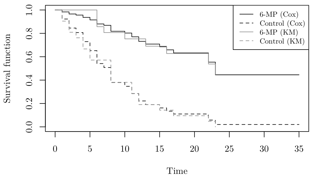

Fitting Cox models using R (leuk)

Leukaemia data: survival times are given for 33 patients who died from acute myelogenous leukaemia. In R, this can be found in the leuk object in the MASS package.

as_tibble(leuk)

# A tibble: 33 × 3
     wbc ag       time
   <int> <fct>   <int>
 1  2300 present    65
 2   750 present   156
 3  4300 present   100
 4  2600 present   134
 5  6000 present    16
 6 10500 present   108
 7 10000 present   121
 8 17000 present     4
 9  5400 present    39
10  7000 present   143
# ℹ 23 more rows

Fitting Cox models using R (leuk)

Using the coxph() and Surv() from the survival package, we can fit a Cox regression model for leuk as follows (using a dummy variable for ag and a natural logarithm of wbc as covariates)

leuk.cox <- coxph(Surv(time) ~ ag + log(wbc), data = leuk)
summary(leuk.cox)

Call:
coxph(formula = Surv(time) ~ ag + log(wbc), data = leuk)

  n= 33, number of events= 33 

            coef exp(coef) se(coef)     z Pr(>|z|)   
agpresent -1.069     0.343    0.429 -2.49   0.0128 * 
log(wbc)   0.368     1.444    0.136  2.70   0.0069 **
---
Signif. codes:  0 '***' 0.001 '**' 0.01 '*' 0.05 '.' 0.1 ' ' 1

          exp(coef) exp(-coef) lower .95 upper .95
agpresent     0.343      2.913     0.148     0.796
log(wbc)      1.444      0.692     1.106     1.886

Concordance= 0.726  (se = 0.047 )
Likelihood ratio test= 15.6  on 2 df,   p=4e-04
Wald test            = 15.1  on 2 df,   p=5e-04
Score (logrank) test = 16.5  on 2 df,   p=3e-04

Fitting Cox models using R (leuk) (Gap on page 70)

The significance of both explanatory variables is immediately obvious from the two p-values \(0.01276\) and \(0.0068\). Strictly, we should formal model selection using either backwards or forwards selection, or using information criteria (see MATH2010).

The estimated coefficient for ag is \(-1.06905\). This means ag being present is estimated to increase the hazard by a factor of \[ \exp \left(-1.06905\right) = 0.34333, \] relative to ag being absent, i.e. ag being present reduces the hazard.

The estimated coefficient for log(wbc) is \(0.3677\). This \(\log(\text{wbc})\) increasing by one unit is estimated to increase the hazard by a factor of \[ \exp\left(0.3677\right) = 1.44441, \] i.e. the higher the wbc, the higher the hazard.

Fitting Cox models using R (leuk)

Similarly to before, we can plot the estimated survival functions as follows.

par(family = "Latin Modern Roman 10", mar = c(5.1, 4.1, 0.5, 2.1))

leuk.S <- survfit(leuk.cox, newdata = data.frame(ag  = c("present", "present", "absent", "absent"), 
                                                 wbc = c(750, 100000, 750, 100000)))

plot(leuk.S, ylab= "Survival function", xlab = "Time", lty = c(1, 2, 1, 2), col = c(1, 1, 8, 8))
legend("topright", lty = c(1, 2, 1, 2), col = c(1, 1, 8, 8), 
legend = c("Present (750)", "Present (100,000)","Absent  (750)", "Absent  (100,000)"), cex = 0.8)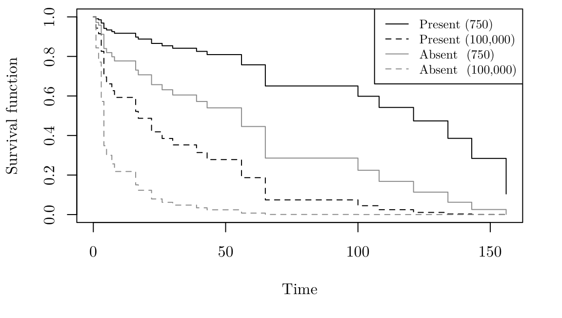

Checking proportional hazards (Gap on page 72)

The assumption that covariates affect the response through proportional hazards is a strong one and should be checked where possible.

Recall that the survival function for \(T_i\) can be written as \[ S_{T_i}(t) = S_0(t)^{\exp \left( \mathbf{x}_i^{\top} \boldsymbol{\beta} \right)}. \] Taking the complementary log-log of both sides \[ \begin{eqnarray*} \log \left( - \log S_{T_i}(t) \right) & = & \log \left( - \exp \left( \mathbf{x}_i^{\top} \boldsymbol{\beta} \right) \log S_0(t) \right)\\ & = & \mathbf{x}_i^{\top} \boldsymbol{\beta} + \log\left(- \log S_0(t) \right). \end{eqnarray*} \]

Checking proportional hazards (Gap on page 72)

Consider units \(i=1\) and \(i=2\) who differ only in the \(j\)-th covariate. Then, \[ \begin{eqnarray*} \mathbf{x}_1^{\top} \boldsymbol{\beta} & = & \sum_{l=1}^k x_{1l}\beta_l = x_{1j} \beta_j + \sum_{l \ne j} x_{1l}\beta_l\\ \mathbf{x}_2^{\top} \boldsymbol{\beta} & = & x_{2j} \beta_j+ \sum_{l \ne j} x_{2l}\beta_l \end{eqnarray*} \] and \[ \begin{eqnarray*} \mathbf{x}_1^{\top} \boldsymbol{\beta} - \mathbf{x}_2^{\top} \boldsymbol{\beta} &=& x_{1j} \beta_j + \sum_{l \ne j} x_{1l}\beta_l - x_{2j} \beta_j- \sum_{l \ne j} x_{2l}\beta_l\\ & = & (x_{1j}-x_{2j}) \cdot \beta_j \end{eqnarray*} \] since \(\sum_{l \ne j} x_{1l}\beta_l = \sum_{l \ne j} x_{2l}\beta_l\).

Checking proportional hazards (Gap on page 72)

Now \[ \log \left( - \log S_{T_1}(t) \right) - \log \left( - \log S_{T_2}(t) \right) = (x_{1j}-x_{2j})\cdot \beta_j \] which does not depend on \(t\).

That means if we were to plot \(\log \left( - \log S_{T_1}(t) \right)\) and \(\log \left( - \log S_{T_2}(t) \right)\) against \(t\) we should get two parallel lines (if the assumption of proportional hazards is correct).

Therefore, a strategy for checking proportional hazards for covariate \(x_j\) is

• Partition the data according to each distinct \(x_j\) value observed
• Fit a separate proportional hazards model (including all other covariates) to each subset
• The estimates of \(\log \left( - \log S_{T}(t) \right)\) for those separate models will be parallel if the proportional hazards assumption holds for \(x_j\).

Clearly this is only practical if \(x_j\) has few distinct values (typically if \(x_j\) is a factor).

Checking proportional hazards

The following R code produces the plot for the gehan dataset, where \(x_j\) corresponds to treat.

logmlog <- function(x) { log(-log(x)) }

par(family = "Latin Modern Roman 10", mar = c(5.1, 4.1, 0.5, 2.1))

gehan.cox1 <- coxph(Surv(time, event = cens) ~ 1, data = gehan[gehan$treat=="control", ])
gehan.cox2 <- coxph(Surv(time, event = cens) ~ 1, data = gehan[gehan$treat=="6-MP",    ])

gehan.S1<- survfit(gehan.cox1)
gehan.S2<- survfit(gehan.cox2)

plot(gehan.S1, ylab= "log(–log(S(t)))", xlab = "Time", fun = logmlog, conf.int = FALSE, xlim = range(gehan$time), lty = 2)
lines(gehan.S2, fun = logmlog, conf.int = FALSE, lty = 1)
legend("bottomright", lty = c(2, 1), legend = c("Control", "6-MP"), cex = 0.8)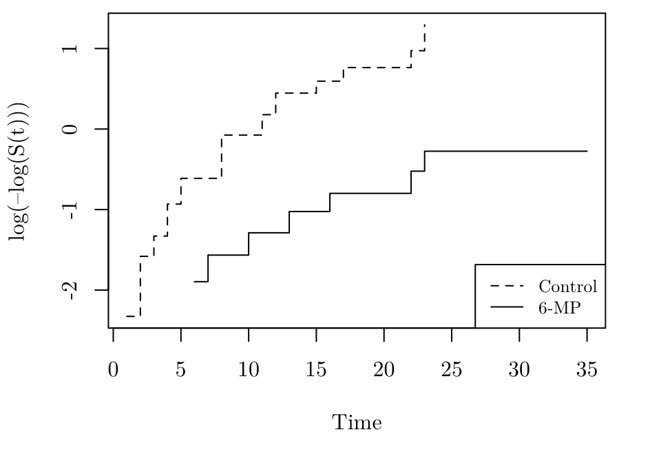

Checking proportional hazards

The following R code produces the plot for the leuk dataset, where \(x_j\) corresponds to ag.

logmlog <- function(x) { log(-log(x)) }

par(family = "Latin Modern Roman 10", mar = c(5.1, 4.1, 0.5, 2.1))

leuk.cox1 <- coxph(Surv(time) ~ log(wbc), data = leuk[leuk$ag == "absent",  ])
leuk.cox2 <- coxph(Surv(time) ~ log(wbc), data = leuk[leuk$ag == "present", ])

leuk.S1 <- survfit(leuk.cox1, newdata = data.frame(wbc = mean(leuk$wbc)))
leuk.S2 <- survfit(leuk.cox2, newdata = data.frame(wbc = mean(leuk$wbc)))

plot(leuk.S1, ylab = "log(–log(S(t)))", xlab = "Time", fun = logmlog, conf.int = FALSE, xlim = range(leuk$time), lty = 1)
lines(leuk.S2, fun = logmlog, conf.int = FALSE, lty = 2)
legend("bottomright", lty = c(1,2), legend = c("Absent","Present"), cex = 0.8)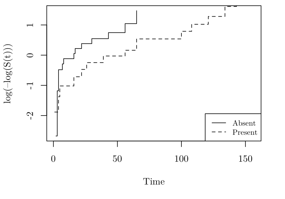

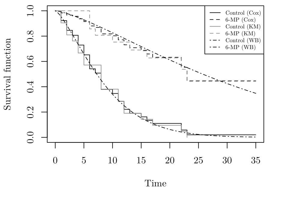
AF and parametric models (Gap on page 74)

We have focused on semiparametric models, where the parameters \(\boldsymbol{\beta}\) do not completely specify the survival distribution.

Fully parametric survival regression models do exist.

For example, consider a Weibull model, with \(T_i \sim \mathrm{Weibull}(\alpha, \theta_i)\) (we changed the scale parameter to \(\theta\) to stop confusion with the \(\boldsymbol{\beta}\) regression parameters). The shape parameter \(\alpha\) is the same for all units but the scale parameter \(\theta_i\) is unit-specific depending on the explanatory variables as follows \[ \begin{eqnarray*} \theta_i & = & 1/\exp\left( \eta_i \right) = \exp\left( - \eta_i \right) = \exp\left( - \beta_0 - \mathbf{x}_i^{\top} \boldsymbol{\beta} \right) = \exp\left( - \beta_0 - \sum_{j=1} x_{ij} \beta_j \right). \end{eqnarray*} \] Now suppose \(T_{0i} \sim \mathrm{Weibull}(\alpha,1)\), then \[ T_i = \exp \left(\eta_i \right)\cdot T_{0i}, \] which can be shown using the properties in Section 4.2.1. The survival functions for \(T_{0i}\) and \(T_i\) are \[ S_{T_{0i}}(t) = \exp \left( -t^\alpha \right) ~~~~~\text{and}~~~~~ S_{T_{i}}(t) = \exp \left( - \left( \exp\left(-\eta_i\right) t \right)^\alpha \right). \]

AF and parametric models (Gap on page 74)

We see that the effect on the distribution of \(T_i\) of the explanatory variables, through \(\eta_i\) is to shrink (or stretch) the time axis, resulting in correspondingly longer (shorter) failure times.

This is called an accelerated failure time (AFT) model (or accelerated life model), and is generally expressed through the survival function \[ S_{T_i}(t)=S_0\left(t \cdot \exp (-\eta_i)\right) \] for some baseline survival function \(S_0\).

Although it is possible to consider semiparametric models (with \(S_0\) not from a standard family) it is more usual to use fully parametric accelerated failure models.

Families of accelerated failure models

\[ T_i=\exp(\eta_i)\cdot T_{0i}~~~\qquad\mbox{where}\qquad~~~ \eta_i=\beta_0+\mathbf{x}_i^{\top}{\boldsymbol{\beta}}. \]

\(T_{0i}\)		\(T_i\)
\(\mathrm{Exp}(1)\)		\(\mathrm{Exp}(\exp[-\eta_i])\)
\(\mathrm{Weibull}(\alpha, 1)\)		\(\mathrm{Weibull}(\alpha, \exp[-\eta_i])\)
\(\mathrm{Loglogistic}(\alpha, 1)\)		\(\mathrm{Loglogistic}(\alpha, \exp[-\eta_i])\)
\(\mathrm{Lognormal}(0, \sigma^2)\)		\(\mathrm{Lognormal}(\eta_i, \sigma^2)\)

Estimating accelerated failure models

For any parametric AFT model, we know the form of \(S_{T_i}\) and \(f_{T_i}\), so we can write down the likelihood \[ L(\theta)=\prod_{i:d_i=1} f_{T_i}(t_i;\theta)\prod_{i:d_i=0} S_{T_i}(t_i;\theta) \] where \(\theta\) comprises the regression parameters \(\beta_0\) and \(\boldsymbol{\beta}\) which enter into the computation of \(\eta_i\) and any other parameters, such as \(\alpha\).

Estimation is performed by maximum likelihood, to obtain \((\hat\beta_0,\,\hat{\boldsymbol{\beta}})\) etc. with standard errors computed in the usual way.

Maximisation must be done numerically (e.g. using R).

Example: Weibull AFT model (gehan)

The R code below fits a Weibull AFT model with a dummy variable for treatment.

gehan.wb <- survreg(Surv(time, event = cens) ~ treat, data = gehan)
summary(gehan.wb)

Call:
survreg(formula = Surv(time, event = cens) ~ treat, data = gehan)
              Value Std. Error     z       p
(Intercept)   3.516      0.252 13.96 < 2e-16
treatcontrol -1.267      0.311 -4.08 4.5e-05
Log(scale)   -0.312      0.147 -2.12   0.034

Scale= 0.732 

Weibull distribution
Loglik(model)= -106.6   Loglik(intercept only)= -116.4
    Chisq= 19.65 on 1 degrees of freedom, p= 9.3e-06 
Number of Newton-Raphson Iterations: 5 
n= 42 

Confusingly, R uses the following parameterisation for the shape parameter \(\hat{\alpha} = \frac{1}{\mathtt{scale}}\).

The estimates are \(\hat{\beta}_0 = 3.516\), \(\hat{\beta}_1 = -1.267\), and \(\hat{\alpha} = 1.366\).

The estimate of \(\beta_1\) is negative meaning the treatment control will increase the scale parameter \(\theta\) and increase the hazard (all relative to the 6-MP treatment).

Example: Weibull AFT model (gehan)

The following R code plots the estimated Kaplan-Meier and Cox survival curves. It then adds estimated survival curves from the Weibull model using the curve function.

par(family = "Latin Modern Roman 10", mar = c(5.1, 4.1, 0.5, 2.1))
gehan.wb <- survreg(Surv(time, event = cens) ~ treat, data = gehan)

alpha         <- (1 / gehan.wb$scale)
theta.control <- exp(-gehan.wb$coefficients[1] - gehan.wb$coefficients[2])
theta.6MP     <- exp(-gehan.wb$coefficients[1])

plot(gehan.S, ylab = "Survival function", xlab = "Time", lty = c(1,2))
lines(gehan.km, lty = c(2, 1), col = 8)
curve(expr = exp(-(theta.control * x) ^ alpha), from = 0, to = 35, add = TRUE, lty = 4)
curve(expr = exp(-(theta.6MP * x) ^ alpha),     from = 0, to = 35, add = TRUE, lty = 4)
legend("topright", lty = c(1, 2, 1, 2, 4, 4), col = c(1, 1, 8, 8, 1, 1), legend = c("Control (Cox)", "6-MP (Cox)", "Control (KM)", "6-MP (KM)", "Control (WB)", "6-MP (WB)"), cex = 0.6)

Example: Weibull AFT model (leuk)

The R code below fits a Weibull AFT model with a dummy variable for test result.

leuk.wb <- survreg(Surv(time) ~ ag + log(wbc), data = leuk)
summary(leuk.wb)

Call:
survreg(formula = Surv(time) ~ ag + log(wbc), data = leuk)
              Value Std. Error     z       p
(Intercept)  5.8524     1.3227  4.42 9.7e-06
agpresent    1.0206     0.3781  2.70  0.0069
log(wbc)    -0.3103     0.1313 -2.36  0.0181
Log(scale)   0.0399     0.1392  0.29  0.7745

Scale= 1.04 

Weibull distribution
Loglik(model)= -146.5   Loglik(intercept only)= -153.6
    Chisq= 14.18 on 2 degrees of freedom, p= 0.00084 
Number of Newton-Raphson Iterations: 6 
n= 33