Survival Models (MATH3085/6143)

Chapter 6: Non-parametric Survival Estimation

André Victor Ribeiro Amaral

a.v.ribeiro-amaral@soton.ac.uk

University of Southampton

20/10/2025

Recap

In the last chapter, we

• Defined the likelihood function \(L(\theta)\), showing how to incorporate all censoring types (although we will focus on right-censored data only).

• Identified Maximum Likelihood Estimation (MLE) as the primary method for finding the parameter estimates \(\hat{\theta}\) in parametric survival models by maximizing the log-likelihood function, \(\ell(\theta)\).

• Derived the MLE for the Exponential model.

• Estimated parameters for more complex models (e.g., Weibull) using numerical methods. We also compared the results with flexsurvreg() (from flexsurv).

Chapter 6: Non-parametric Survival Estimation

Introduction

Frequently, we want to estimate the distribution of \(T\) for the (i.i.d.) homogeneous model based on

• observations \(t_1, \cdots ,t_n\)
• with (right-) censoring indicators \(d_1, \cdots ,d_n\),

without assuming a particular parametric family for \(f_T\).

The likelihood is given by \[ L(\theta)=\prod_{i:d_i=1} f_T(t_i; \theta)\prod_{i:d_i=0} S_T(t_i; \theta) \] and this can be made infinitely large by concentrating \(f_T\) in infinitesimally narrow regions around each observed \(t_i\) (i.e. those for which \(d_i=1\)). That is, if we only require \(f_T(t) \ge 0\) for all \(t \in \mathbb{R}_+\) and \(\int_0^{\infty}f_T(t)dt = 1\), without any additional smoothness or parametric constraints, then the likelihood is unbounded.

To resolve this, the non-parametric maximum likelihood estimate of the survival distribution is taken to be a discrete distribution supported on the observed failure times \(\{t_i: d_i=1\}\).

Discrete survival distributions (Gap on page 45)

A discrete survival variable \(T\) takes values in a sample space \(0<t'_1<t'_2<\cdots <t'_m<\infty\) and is defined by any of

• Probability function

\[ f_i =\mathbb{P}(T=t'_i), \qquad \text{for}~~ i=1, \cdots, m. \]

• Survival function

\[ \begin{eqnarray*} S(t)=\mathbb{P}(T>t)&=&1-\sum_{j:t'_j\le t} f_j\\ &\equiv& s_i, \qquad \text{for}~~ t\in[t'_i,t'_{i+1}) ~~\text{and}~~ i=0, \cdots ,m, \end{eqnarray*} \] where \(t'_0 \equiv 0\) and \(t'_{m+1} \equiv \infty\).

Discrete survival distributions (Gap on page 45)

• Hazard function

\[ \begin{eqnarray*} h_i & = & \mathbb{P}(T=t'_i|T\ge t'_i) = \frac{\mathbb{P}(T = t'_i \quad \mbox{and} \quad T\ge t'_i)}{\mathbb{P}(T\ge t'_i)} = \frac{\mathbb{P}(T = t'_i)}{\mathbb{P}(T\ge t'_i)} = \frac{f_i}{\mathbb{P}(T > t'_{i-1})}\\ & = & \frac{f_i}{s_{i-1}} \end{eqnarray*} \]

We have \(s_0=1\) and

\[ \begin{eqnarray*} s_i & = & \mathbb{P}(T > t_i') = 1 - \mathbb{P}(T \le t_i') = 1 - \left(\mathbb{P}(T \le t_{i-1}') + f_i \right)\\ & =& \mathbb{P}(T>t_{i-1}') - f_i = s_{i-1} - f_i = s_{i-1}-h_i s_{i-1} = s_{i-1}(1-h_i ) \end{eqnarray*} \]

Therefore, \[ s_i=\prod_{j=1}^i (1-h_j)\qquad{\rm and}\qquad f_i=h_i\prod_{j=1}^{i-1} (1-h_j) \]

It is best to describe the survival distributions through \(\{h_i\}\), which are simply constrained to be in \([0,1]\), rather than \(\{f_i\}\) or \(\{s_i\}\) (which have more complex constraints).

Likelihood (Gap on page 48)

We will now connect these functions in the discrete case to the likelihood discussed in the previous chapter. To do so,

• Let \(0<t'_1<t'_2<\cdots <t'_m<\infty\) denote the distinct observed failure times observed in our sample \(\{t_1,\cdots , t_n\}\).

• \(t'_0=0\) and \(t'_{m+1}=\infty\).

• \(d'_i\) is the number of failures observed at \(t'_i,\; ( i=1,\cdots ,m)\), so

\[ \sum_{i=1}^m d'_i = \sum_{i=1}^n d_i=d_+. \]

• \(c_i\; ( i=0,\cdots ,m)\) is the number of censored observations with censoring times between \(t'_i\) and \(t'_{i+1}\).

Likelihood (Gap on page 48)

The likelihood is given by

\[ \begin{eqnarray*} L(\theta)=\prod_{i=1}^m f_i^{d'_i} \prod_{i=0}^m s_i^{c_i} &=&\prod_{i=1}^m \left[h_i\prod_{j=1}^{i-1} (1-h_j)\right]^{d'_i} \prod_{i=1}^m \left[\prod_{j=1}^i (1-h_j)\right]^{c_i}\\ &=&\prod_{i=1}^m \left[\left(\frac{h_i}{1-h_i}\right)^{d'_i}\prod_{j=1}^i (1-h_j)^{d'_i+c_i}\right]\\ &=&\left[\prod_{i=1}^m \left(\frac{h_i}{1-h_i}\right)^{d'_i}\right]\prod_{i=1}^m\prod_{j=1}^i (1-h_j)^{d'_i+c_i}\\ &=&\left[\prod_{i=1}^m \left(\frac{h_i}{1-h_i}\right)^{d'_i}\right]\prod_{i=1}^m\prod_{j=i}^m (1-h_i)^{d'_j+c_j}\\ &=&\left[\prod_{i=1}^m \left(\frac{h_i}{1-h_i}\right)^{d'_i}\right]\prod_{i=1}^m(1-h_i)^{\sum_{j=i}^m (d'_j+c_j)}\\ \end{eqnarray*}. \]

Likelihood (Gap on page 48)

The log-likelihood is given by

\[ \ell(\theta)=\sum_{i=1}^m \left[d'_i\log h_i -d'_i\log(1-h_i) +\log (1-h_i)\sum_{j=i}^m (d'_j+c_j)\right], \]

so

\[ \frac{\partial\ell}{\partial h_i}=\frac{d'_i}{h_i}+ \frac{d'_i}{1-h_i} - \frac{\sum_{j=i}^m (d'_j+c_j)}{1-h_i}. \] and

\[ \begin{eqnarray*} &&\frac{d'_i}{\hat{h}_i}+ \frac{d'_i-\sum_{j=i}^m (d'_j+c_j)}{1-\hat{h}_i} ~~\overset{\text{SET}}{=}~~ 0\\ &\text{implying}\qquad&\hat{h}_i=\frac{d'_i}{\sum_{j=i}^m (d'_j+c_j)},\qquad i=1,\cdots,m. \end{eqnarray*} \]

The Kaplan-Meier estimator (Gap on page 49)

The discrete hazard MLE is \[ \hat{h}_i=\frac{d'_i}{r_i},\qquad i=1,\cdots, m, \qquad \text{ where } \qquad r_i=\sum_{j=i}^m (d'_j+c_j) \] is the number at risk (of failure) at \(t'_i\).

The hazard at each \(t'_i\) is therefore estimated by the observed number of failures at \(t'_i\) as a proportion of the number at risk at \(t'_i\).

The corresponding estimator of the survival function \[ \hat{S}(t)=\prod_{j=1}^i (1-\hat{h}_j)=\prod_{j=1}^i \left(1-\frac{d'_j}{r_j}\right)\qquad t\in[t'_i,t'_{i+1}), \quad i=0,\cdots ,m \] is called the Kaplan-Meier (or product-limit) estimator.

Kaplan-Meier estimator

Gehan data: remission times (in weeks) from a clinical trial of 42 leukaemia patients. Patients matched in pairs and randomised to 6-mercaptopurine (drug) or control (from MASS package).

Using the survfit() and Surv() functions from the survival package, we can compute the KM curves as follows

gehanControl <- survfit(Surv(time = gehan$time[gehan$treat == "6-MP"   ], event = gehan$cens[gehan$treat == "6-MP"]   ) ~ 1)
gehan6mp     <- survfit(Surv(time = gehan$time[gehan$treat == "control"], event = gehan$cens[gehan$treat == "control"]) ~ 1)

par(family = "Latin Modern Roman 10", mar = c(1.85, 4.1, 0.5, 2.1))
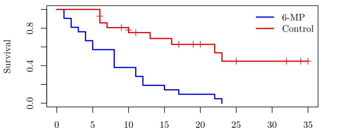
plot( gehan6mp,     mark.time = TRUE, conf.int = FALSE, col = "blue", lwd = 2, xlab = "Time (weeks)", ylab = "Survival", main = NA, xlim = c(0, 35))
lines(gehanControl, mark.time = TRUE, conf.int = FALSE, col = "red",  lwd = 2)
legend("topright", legend = c("6-MP", "Control"), col = c("blue", "red"), lwd = 2, bty = "n")

# Alternatively, one can use `treat` as a covariate. This would produce the same plot.
# gehan.km <- survfit(Surv(time, cens) ~ treat, data = gehan)
# plot(gehan.km, xlab = "Time (weeks)", ylab = "S(time)", lty = c(1, 2), xlim = c(0, 35))

Notes on Kaplan-Meier estimator (Gap on page 50)

• Although the Kaplan-Meier estimator represents a discrete survival distribution, we use it to estimate \(S_T(t)\) for continuous \(T\).

• For censored times tied with uncensored times, we treat the censored times as infinitessimally larger than the uncensored ones with which they are tied (so \(c_i\) includes observations censored at \(t'_i\)).

• If the largest time is censored (so \(c_m>0\)), then the Kaplan-Meier estimator is positive at the largest uncensored time and therefore the estimated survivor function is nowhere zero.

• Sometimes, it is informative to plot \(\log{S}(t)\), recalling that the hazard function \(h(t)\) is equal to \(-\frac{\mathrm{d}}{\mathrm{d}t}\log S(t)\). Hence \(\log{S}(t)\) is linear for exponentially distributed data (constant hazard).

Kaplan-Meier estimate by hand (Gap on page 50)

Consider the following survival times \(\mathbf{t} = \left(3, 4, 6^*, 8, 8, 10\right)\). There are \(m=4\) distinct observed survival times.

\(i\)	\(t_i\)	\(t_{i+1}\)	\(r_i\)	\(d_i'\)	\(c_i\)	\(\hat{S}(t)\)
\(0\)	\(0\)	\(3\)	\(6\)	\(0\)	\(0\)	\(1\)
\(1\)	\(3\)	\(4\)	\(6\)	\(1\)	\(0\)	\(\frac{5}{6}\)
\(2\)	\(4\)	\(8\)	\(5\)	\(1\)	\(1\)	\(\frac{2}{3}\)
\(3\)	\(8\)	\(10\)	\(3\)	\(2\)	\(0\)	\(\frac{2}{9}\)
\(4\)	\(10\)	\(\infty\)	\(1\)	\(1\)	\(0\)	\(0\)

par(family = "Latin Modern Roman 10", mar = c(5.1, 4.1, 0.5, 2.1))

plot(0, 0, type="l", xlim=c(0,12), ylim=c(0,1), xlab = "Time", ylab = "S(time)")
segments(x0 = c(0, 3, 4, 8, 10), x1=c(3, 4, 8, 10, 12), y0=c(1, 5/6, 2/3, 2/9,0), y1 = c(1, 5/6, 2/3, 2/9, 0), lwd = 2, col = "red")
segments(x0 = c(3, 4, 8, 10),    x1=c(3, 4, 8, 10),     y0=c(1, 5/6, 2/3, 2/9  ), y1 = c(5/6, 2/3, 2/9, 0   ), lwd = 2, col = "red")

Kaplan-Meier with R

As before, we can compute it in R using the survival package.

par(family = "Latin Modern Roman 10", mar = c(5.1, 4.1, 2.5, 2.1))

time <- c(3, 4, 6, 8, 8, 10)
cens <- c(1, 1, 0, 1, 1, 1 )

km <- survfit(Surv(time, cens) ~ 1)

par(mfrow=c(1,2))
plot(km, conf.int = FALSE, xlab = "Time", ylab = "S(time)", main = "Without 'censoring marks' and CI")
plot(km, mark.time = TRUE, xlab = "Time", ylab = "S(time)", main =    "With 'censoring marks' and CI")

Standard Errors and CIs (Gap on page 55)

The standard error of the Kaplan-Meier estimator is given by Greenwood’s formula (i.e., a formula used to approximate the variance of the Kaplan-Meier estimator) \[ \text{se}[\hat{S}(t)]^2=\hat{S}(t)^2 \sum_{j=1}^i {{d'_j}\over{r_j(r_j-d'_j)}}\qquad t\in[t'_i,t'_{i+1}), \quad i=0,\cdots ,m \]

Using a normal approximation for the sampling distribution of \(\hat{S}(t)\), we can obtain endpoints of an approximate \((1-\alpha)\%\) confidence interval for \(S(t)\) as \[ \hat{S}(t)\pm z_{\left(1-\frac{\alpha}{2}\right)} \cdot \text{se}[\hat{S}(t)]. \]

Standard Errors and CIs (Gap on page 55)

Better confidence intervals are often obtained on the log scale, using \[ \text{se}[\log\hat{S}(t)]^2= \sum_{j=1}^i {{d'_j}\over{r_j(r_j-d'_j)}}\qquad t\in[t'_i,t'_{i+1}), \quad i=0,\cdots ,m \] to give endpoints of an alternative \((1-\alpha)\%\) confidence interval as \[ \hat{S}(t)\cdot \exp\left\{\pm z_{\left(1-\frac{\alpha}{2}\right)}\cdot \text{se}[\log\hat{S}(t)]\right\}. \]

The Nelson-Aalen estimator (Gap on page 56)

The Nelson-Aalen estimator estimates the cumulative hazard function \(H(t)\) by integrating (summing) the discrete hazard estimators \(\hat{h}_i=d'_i/r_i\), and is given by

\[ \hat{H}(t)=\sum_{j=1}^i \hat{h}_j=\sum_{j=1}^i \frac{d'_j}{r_j}\qquad t\in[t'_i,t'_{i+1}), \quad i=0,\cdots ,m. \]

As \(S(t)=\exp \{-H(t)\}\), the Nelson-Aalen estimator provides an estimator of \(S(t)\) as

\[ \hat{S}(t)= \exp\left(-\sum_{j=1}^i\frac{d'_j}{r_j}\right)= \prod_{j=1}^i\exp\left(-\frac{d'_j}{r_j}\right)\qquad t\in[t'_i,t'_{i+1}), \quad i=0,\cdots,m \]

which is sometimes called the Fleming-Harrington estimator.

Notes on Nelson-Aalen estimator (Gap on page 57)

Plotting \(\log[{\hat H}(t)]\) against \(\log(t)\) checks whether a Weibull model might fit the data, as for the Weibull, \[ H(t)=(\beta t)^\alpha\qquad\Rightarrow\qquad \log [H(t)]=\alpha\log(\beta)+\alpha\log(t), \] so for Weibull data, we would expect \(\log {\hat H}(t)\) to be linear in \(\log(t)\), with gradient \(\alpha\).

If \(d'_i/r_i\) is small (typical for smaller values of \(t\)) then the Kaplan-Meier and Fleming-Harrington estimators of \(S(t)\) will be close, as \[ \begin{eqnarray*} \exp\left(-\frac{d'_j}{r_j}\right)&=&1-\frac{d'_j}{r_j}+\frac{1}{2}\left(\frac{d'_j}{r_j}\right)^2 -\cdots\\ &\approx& 1-\frac{d'_j}{r_j}. \end{eqnarray*} \]