Survival Models (MATH3085/6143)

Chapter 5: Survival models: parameter estimation

André Victor Ribeiro Amaral

a.v.ribeiro-amaral@soton.ac.uk

University of Southampton

09/10/2025

Recap

In the last chapter, we

• Reviewed Key Parametric Distributions: we focused on the Exponential, Weibull, Log-Logistic, LogNormal, and Gompertz (and Makeham in PC 1) distributions, which all have a non-negative domain suitable for modeling time \(T\).

• Interpreted the different hazard function shapes \(h_T\) for each distribution.

• Established the critical relationship between the Exponential and Weibull distributions, as well as their transformations.

Chapter 5: Survival models: parameter estimation

Introduction

We start by considering models for a homogenous population of survival times, from which we have observed a sample \(\mathbf{t} = \left(t_1,\dots t_n\right)\).

Some of the observations may be censored.

• Here, we will only consider right censoring (most common) only.
• Extension to other forms of censoring is possible.

Let \(d_1,\cdots ,d_n\) be a set of censoring indicators, with

\[ d_i=\left\{\begin{array}{ll} 0&{\rm unit~}i{\rm~was~censored~at~}t_i{\rm~so~actual~failure ~time~}>t_i\\ 1&{\rm failure~of~unit~}i{\rm~was~observed~at~}t_i\end{array}\right. \]

Therefore \(t_1, \cdots, t_n\) are (possibly censored) observations of i.i.d. random variables \(\mathbf{T} = \left(T_1,\cdots,T_n\right) \equiv T\).

Parametric models

A parametric model for \(T\) specifies the p.d.f \(f_T\), apart from the values of a (small) number of unknown parameters, which we denote by \(\boldsymbol{\theta}\).

For example, for a Weibull model, \(\boldsymbol{\theta}\) comprises the shape and scale parameters \(\alpha\) and \(\beta\), i.e. \(\boldsymbol{\theta} = (\alpha,\beta)\).

We write \(f_T(t;\boldsymbol{\theta})\) to recognise the dependence of the p.d.f. \(f_T\) on \(\boldsymbol{\theta}\).

Similarly, for the survivor \(S_T(t;\boldsymbol{\theta})\) and hazard \(h_T(t;\boldsymbol{\theta})\) functions on \(\boldsymbol{\theta}\).

Parametric models

Estimating the distribution of \(T\) then simply involves estimating \(\boldsymbol{\theta}\).

Once we have an estimate \(\hat{\boldsymbol{\theta}}\) of \(\boldsymbol{\theta}\), we can obtain the corresponding estimates \(S_T(t;\hat{\boldsymbol{\theta}})\) and \(h_T(t;\hat{\boldsymbol{\theta}})\) of the survival and hazard functions.

Typically, we use maximum likelihood estimation to obtain \(\hat{\boldsymbol{\theta}}\) in a parametric model.

Maximum likelihood

Maximum likelihood estimation is a general method for parameter estimation with many good properties (see MATH3044 for more).

Initially consider a scalar parameter \(\theta\).

The maximum likelihood estimator (MLE) \(\hat{\theta}\) maximises the likelihood \(L(\theta)\).

The likelihood \(L(\theta)\) is simply the joint probability (density) of the observed data, treated as a function of the unknown \(\theta\).

Maximum likelihood

The likelihood \(L(\theta)\) is simply the joint probability (density) of the observed data, treated as a function of the unknown \(\theta\).

Assuming i.i.d. observations with no censoring \[ L(\theta)=\prod_{i=1}^n f_T(t_i;\theta), \] as the joint PDF of independent variables is just the product of their individual (marginal) PDFs.

Censored data likelihood (Gap on page 37)

For a right censored observation, \(t_i\) is not an observed value of \(T_i\), but an interval \((t_i, \infty)\) for \(T_i\).

Hence, the appropriate contribution to the likelihood for a censored \(t_i\) is not \(f_T(t_i;\theta)\), but rather \(\mathbb{P}(T_i>t_i)=S_T(t_i)\).

Assuming i.i.d. observations with (right) censoring indicators \(d_1,\cdots ,d_n\), \[ L(\theta)=\prod_{i:d_i=1} f_T(t_i;\theta)\prod_{i:d_i=0} S_T(t_i;\theta) \]

This is a product of two terms: one for the exact observations and one for the censored observations.

Censored data likelihood (Optional)

Let \(d_i\), \(c_{\text{right},i}\), \(c_{\text{left},i}\), and \(c_{\text{interval},i}\) be a set of four indicators for the \(i\)-th observation, where exactly one is equal to \(1\), and the others are \(0\).

Indicator	Condition	Contribution
\(d_i\)	Failure was observed at \(t_i\).	\(f_T(t_i;\theta)\)
\(c_{\text{right},i}\)	Unit was right-censored at \(t_i\).	\(S_T(t_i;\theta)\)
\(c_{\text{left},i}\)	Unit was left-censored at \(t_i\).	\(F_T(t_i;\theta)\)
\(c_{\text{interval},i}\)	Unit was interval-censored on \((t_{1,i}, t_{2,i})\).	\(S_T(t_{1,i};\theta) - S_T(t_{2,i};\theta)\)

Assuming i.i.d. observations, the complete likelihood function is

\[ L(\theta) = \prod_{i:d_i=1} f_T(t_i;\theta) \prod_{i:c_{\text{right},i}=1} S_T(t_i;\theta) \prod_{i:c_{\text{left},i}=1} F_T(t_i;\theta) \prod_{i:c_{\text{interval},i}=1} \left[S_T(t_{1,i};\theta) - S_T(t_{2,i};\theta)\right]. \]

Maximum likelihood properties (Gap on page 38)

Usually, it is easier to maximise the log-likelihood \(\ell(\theta)=\log L(\theta)\).

For large samples, we have the asymptotic approximation (not proved here) \[ \hat{\theta}\;\;\stackrel{\text{approx.}}{\sim}\; \text{Normal}(\theta, I(\theta)^{-1}), \] where \[ I(\theta)=\mathbb{E}\left[-\frac{\partial^2}{\partial\theta^2} \ell(\theta)\right] \] is called the Fisher information. A multi-parameter extension of this result exists but is outside the scope of this module (you will see that in MATH3044).

Maximum likelihood properties (Gap on page 38)

In large samples, the MLE is approximately unbiased, and we can construct \(100(1-\alpha)\%\) confidence intervals as \[ \hat{\theta}\pm z_{\left(1-\frac{\alpha}{2}\right)} \cdot \text{se}(\hat{\theta}) \] where \(\text{se}(\hat{\theta})\), the standard error, is given by \[ \text{se}(\hat{\theta})=\left[I(\hat{\theta})^{-1}\right]^{\frac{1}{2}} \] and \(z_{\left(1-\frac{\alpha}{2}\right)}\) is the \(\left(1-\frac{\alpha}{2}\right)\)-th quantile of the standard normal (computed, e.g., using R).

Maximum likelihood properties

These quantiles can be numerically calculated using the R function qnorm(). For instance, for \(\alpha= 0.1\), \(\alpha = 0.05\) and \(\alpha = 0.01\).

qnorm(0.950)

[1] 1.645

qnorm(0.975)

[1] 1.96

qnorm(0.995)

[1] 2.576

which would be needed for \(90\%\), \(95\%\) and \(99\%\) confidence intervals, respectively.

Exponential model likelihood (Gap on page 40)

Suppose that we want to fit an exponential model to our data, so \[ \begin{eqnarray*} L(\beta)&=&\prod_{i:d_i=1} f_T(t_i;\beta)\prod_{i:d_i=0} S_T(t_i;\beta)\\[5pt] &=&\prod_{i:d_i=1} \beta\exp\left(-\beta t_i\right)\prod_{i:d_i=0} \exp\left(-\beta t_i\right)\\[5pt] &=&\beta^{d_+}\exp\left(-\beta \sum_{i=1}^n t_i\right), \end{eqnarray*} \] where \(d_+=\sum_{i=1}^n d_i\) is the number of uncensored observations.

Therefore, the log-likelihood is \[ \ell(\beta)= d_+\log \beta - \beta \sum_{i=1}^n t_i. \]

Exponential model likelihood (Gap on page 40)

The MLE for \(\beta\) in the exponential model maximises \(\ell(\beta)\) and therefore solves \[ 0\;\;=\;\;\frac{\partial}{\partial\beta} \ell(\beta)\;\;=\;\; \frac{d_+}{\beta} - \sum_{i=1}^n t_i. \] Thus, \[ \frac{d_+}{\hat{\beta}}= \sum_{i=1}^n t_i \qquad\Rightarrow\qquad \hat\beta=\frac{d_+}{\sum_{i=1}^n t_i}. \] so \(\hat{\beta}\) is the number of uncensored observations divided by the sum of the (censored and observed) survival times.

The second derivative of the log-likelihood is \[ \frac{\partial^2}{\partial\beta^2} \ell(\beta)\;\;=\;\; - \frac{d_+}{\beta^2}. \]

Exponential model likelihood (Gap on page 40)

The Fisher information is \[ \begin{eqnarray*} I(\beta) & = & \mathbb{E} \left( - \frac{\partial^2}{\partial\beta^2} \ell(\beta) \right)\\ & = & \mathbb{E} \left( \frac{d_+}{\beta^2}\right) \approx \frac{d_+}{\beta^2}, \end{eqnarray*} \] where \(\mathbb{E}(d_+) = d_+\) is assumed to be \(d_+\) (plug-in approximation).

Therefore, for the Exponential model, the standard error is \[ \begin{eqnarray*} \text{se}(\hat{\beta}) & = & \left[ I(\hat{\beta})^{-1} \right]^{\frac{1}{2}} = \frac{\hat{\beta}}{\sqrt{d_+}}. \end{eqnarray*} \]

Using a Normal approximation, a \(100(1 - \alpha)\%\) confidence interval is \[ \hat{\beta} \pm z_{\left(1-\frac{\alpha}{2}\right)} \cdot \frac{\hat{\beta}}{\sqrt{d_+}}. \]

Gehan data

Remission times (before relapsing), in weeks, from a clinical trial of 42 leukaemia patients. Patients matched in pairs and randomised to 6-mercaptopurine (drug) or control. In R, data is found in the MASS package in the gehan object.

library("MASS")
as_tibble(gehan)

# A tibble: 42 × 4
    pair  time  cens treat  
   <int> <int> <int> <fct>  
 1     1     1     1 control
 2     1    10     1 6-MP   
 3     2    22     1 control
 4     2     7     1 6-MP   
 5     3     3     1 control
 6     3    32     0 6-MP   
 7     4    12     1 control
 8     4    23     1 6-MP   
 9     5     8     1 control
10     5    22     1 6-MP   
# ℹ 32 more rows

We fit exponential models separately to the treatment and control groups.

Gehan data

• 6-MP treatment group

(t1 <- gehan$time[gehan$treat=="6-MP"]) # Remission time      for the `6-MP` group

 [1] 10  7 32 23 22  6 16 34 32 25 11 20 19  6 17 35  6 13  9  6 10

(c1 <- gehan$cens[gehan$treat=="6-MP"]) # Censoring indicator for the `6-MP` group

 [1] 1 1 0 1 1 1 1 0 0 0 0 0 0 1 0 0 1 1 0 0 0

n1 <- length(t1); d1 <- sum(c1) # Total number of observations (exact + censored) and number of exact observation
beta1 <- d1 / sum(t1)   # Estimated parameter for the `6-MP` group
se1 <- beta1 / sqrt(d1) # Standard error      for the `6-MP` group

data.frame(n1 = n1, d1 = d1, beta1 = beta1, se1 = se1)

  n1 d1   beta1      se1
1 21  9 0.02507 0.008357

• control treatment group

(t2 <- gehan$time[gehan$treat=="control"]) # Remission time      for the `control` group

 [1]  1 22  3 12  8 17  2 11  8 12  2  5  4 15  8 23  5 11  4  1  8

(c2 <- gehan$cens[gehan$treat=="control"]) # Censoring indicator for the `control` group

 [1] 1 1 1 1 1 1 1 1 1 1 1 1 1 1 1 1 1 1 1 1 1

n2 <- length(t2); d2 <- sum(c2) # Total number of observations (exact + censored) and number of exact observation
beta2 <- d2/sum(t2)   # Estimated parameter for the `control` group
se2 <- beta2/sqrt(d2) # Standard error      for the `control` group

data.frame(n2 = n2, d2 = d2, beta2 = beta2, se2 = se2)

  n2 d2  beta2     se2
1 21 21 0.1154 0.02518

Gehan data (Gap on page 42)

For the 6-MP treatment group, \(n=21\), \(d_+=9\), and \(\sum_{i=1}^n t_i=359\), so \[ \hat\beta=\frac{9}{359} = 0.025 \qquad{\rm~and~}\qquad \text{se}(\hat{\theta})=\frac{0.025}{\sqrt{9}} =0.08 \] For the control treatment group, \(n=21\), \(d_+=21\) and \(\sum_{i=1}^n t_i=182\), so \[ \hat\beta=\frac{21}{182} = 0.115 \qquad{\rm~and~}\qquad \text{se}(\hat{\beta})=\frac{0.115}{\sqrt{21}} = 0.025 \] Assuming this model, approximate \(95\%\) confidence intervals for \(\beta\) are

• 6-MP

print(paste("[", round(beta1 - qnorm(0.975) * se1, 3), ", ", round(beta1 + qnorm(0.975) * se1, 3), "]", sep = ""))

[1] "[0.009, 0.041]"

• control group

print(paste("[", round(beta2 - qnorm(0.975) * se2, 3), ", ", round(beta2 + qnorm(0.975) * se2, 3), "]", sep = ""))

[1] "[0.066, 0.165]"

Gehan data

The plot below shows the log-likelihood curves for both groups (6-MP and control).

beta_seq <- seq(from = 0.001, to = 0.3, length.out = 1000)
loglik1 <- loglik2 <- rep(0, 1000)
for (b in 1:1000) { loglik1[b] <- d1 * log(beta_seq[b]) - sum(t1) * beta_seq[b]; loglik2[b] <- d2 * log(beta_seq[b]) - sum(t2) * beta_seq[b] }
df_loglik <- data.frame(beta = beta_seq, group1 = loglik1, group2 = loglik2) %>% tidyr::pivot_longer(cols = c(group1, group2), names_to = "Group", values_to = "loglik")

ggplot(df_loglik, aes(x = beta, y = loglik, linetype = Group)) + geom_line(linewidth = 0.6) +
  geom_segment(data = . %>% group_by(Group) %>% filter(loglik == max(loglik)), aes(x = beta, xend = beta, y = -200, yend = loglik, linetype = Group), color = "black", linewidth = 0.6, inherit.aes = FALSE) +
  geom_point(  data = . %>% group_by(Group) %>% filter(loglik == max(loglik)), aes(x = beta, y = loglik), size = 2, inherit.aes = FALSE) +
  labs(x = "parameter", y = "log-likelihood") +
  scale_linetype_manual(values = c("group1" = "solid", "group2" = "dashed"), name = NULL, labels = c("6-MP", "Control")) +
  theme_bw() + theme(legend.position = "right", panel.grid.major = element_blank(), panel.grid.minor = element_blank(), axis.line = element_line(color = "black"), panel.border = element_blank(), text = element_text(size = 16, family = "Latin Modern Roman 10")) + coord_cartesian(ylim = c(min(df_loglik$loglik, na.rm = TRUE) * 1.05, max(df_loglik$loglik, na.rm = TRUE) * 1.05))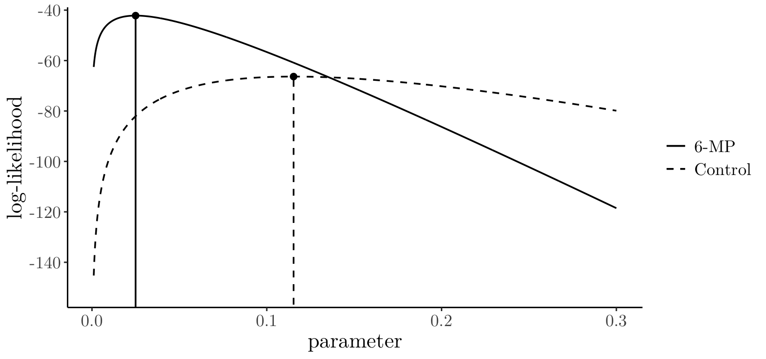

Weibull model likelihood (Gap on page 44)

For a \(\text{Weibull}(\alpha,\beta)\) model, \[ \begin{eqnarray*} L(\alpha,\beta)&=&\prod_{i:d_i=1} f_T(t_i;\alpha,\beta)\prod_{i:d_i=0} S_T(t_i;\alpha,\beta)\\[5pt] &=&\prod_{i:d_i=1} \alpha\beta \left(\beta t \right)^{\alpha-1}\exp\left\{ - \left(\beta t \right)^{\alpha}\right\} \prod_{i:d_i=0} \exp\left\{ - \left(\beta t \right)^{\alpha}\right\}\\[5pt] &=& \alpha^{d_+} \beta^{\alpha d_+} \left( \prod_{i:d_i=1} t_i \right)^{\alpha-1} \exp \left( - \sum_{i=1}^n \left(\beta t_i\right)^{\alpha} \right). \end{eqnarray*} \] Therefore, \[ \ell(\alpha,\beta)= d_+ \log \alpha +\alpha d_+ \log \beta +(\alpha - 1) \sum_{i:d_i=1} \log t_i - \beta^\alpha \sum_{i=1}^n t_i^\alpha. \] Requires numerical solution of \(\frac{\partial\ell}{\partial\alpha}=0,\;\frac{\partial\ell}{\partial\beta}=0\) (use R or similar).

Weibull model likelihood

# Example data
t <- c(2.3, 1.8, 3.2, 2.5, 4.1, 1.2, 3.5, 2.9, 1.6, 3.8)
d <- c(1, 0, 1, 1, 0, 1, 1, 0, 1, 1)  # 1 = observed, 0 = censored

# Log-likelihood for a Weibull model
loglik_weibull_cens <- function(par, t, d) {
  alpha <- par[1]
  beta  <- par[2]
  
  if (alpha <= 0 || beta <= 0) return(-Inf) # Enforce positivity
  
  d_plus <- sum(d)
  term1  <- d_plus * log(alpha)
  term2  <- alpha * d_plus * log(beta)
  term3  <- (alpha - 1) * sum(log(t[d == 1]))
  term4  <- (beta^alpha) * sum(t^alpha) * (-1)
  
  ll <- term1 + term2 + term3 + term4
  return(ll)
}

# Numerical maximisation
fit_manual <- optim(par = c(1, 0.5),  
                    fn = function (par) { -loglik_weibull_cens(par, t, d)},
                    method = "L-BFGS-B", lower = c(1e-6, 1e-6))

fit_manual[c("par", "value")]

$par
[1] 3.0173 0.2985

$value
[1] 12.4

Weibull model likelihood

Now, let’s fit the same model using the flexsurvreg() from the flexsurv package (more about it later).

library("flexsurv")

fit_flex <- flexsurvreg(Surv(t, d) ~ 1, dist = "weibull")

# Extract shape and scale
alpha_hat_flex <- fit_flex$res["shape", "est"]
scale_hat_flex <- fit_flex$res["scale", "est"]

# Convert to our parameterisation
beta_hat_flex <- 1 / scale_hat_flex

c(alpha_hat_flex = alpha_hat_flex, beta_hat_flex = beta_hat_flex)

alpha_hat_flex  beta_hat_flex 
        3.0173         0.2985 

fit_flex$loglik

[1] -12.4

Notice that flexsurvreg() uses a different parameterisation (same as dweibull(); see doc. page 25). In particular, as in ?dweibull, the density of \(\text{Weibull}(\text{shape = }a, \text{scale = }\sigma)\) is \[ f(x)=(a/\sigma)(x/\sigma)^{a−1}\exp(−(x/\sigma)^a). \]