Survival Models (MATH3085/6143)

Chapter 4: Distributions for Survival Models

André Victor Ribeiro Amaral

a.v.ribeiro-amaral@soton.ac.uk

University of Southampton

02/10/2025

Recap

In the last chapter, we

• Established the three core functions needed to model survival time \(T\), namely the density Function \(f_T\), the survival function \(S_T\), and the hazard function \(h_T\).

• Defined the survival function \(S_T\) as the probability of surviving past time \(t\), and found that the expected lifetime \(\mathbb{E}(T)\) equals the area under this curve.

• Defined the hazard function \(h_T\) as the instantaneous event rate at the time \(t\), conditional on prior survival.

• Confirmed all survival functions are linked, meaning specifying any one function completely defines the entire distribution of the survival time \(T\).

Chapter 4: Distributions for Survival Models

Introduction

• We now introduce some distributions which are commonly used in survival models.

• Each of these distributions has domain \((0, \infty)\) so is appropriate as a model for a survival time \(T\).

• In each case, we shall present the density function \(f_T(t)\), the survival function \(S_T(t)\) and the hazard function \(h_T(t)\).

The exponential distribution

The exponential distribution has a single parameter, the rate (scale) \(\beta>0\), is denoted \({\exp}(\beta)\) and has p.d.f. \[ f_T(t)=\beta \exp\left(-\beta t\right), \] survival function \[ S_T(t)=\exp\left(-\beta t\right), \] and hazard function \[ h_T(t)=\beta. \]

If \(T\sim \exp(\beta)\) then \[ \mathbb{E}(T)=\frac{1}{\beta} \qquad{\rm and}\qquad \text{Var}(T)=\frac{1}{\beta^2}. \] Note that the p.d.f. is sometimes parameterised as \(\frac{1}{\gamma} \exp\left(-\frac{t}{\gamma}\right)\), i.e. \(\gamma = 1/\beta\).

The exponential distribution (Gap on page 25)

The survival function is given by \[ \begin{eqnarray*} S_T(t) & = & \int_t^{\infty} f_T(u) \mathrm{d}u\\ & = & \int_t^{\infty}\beta \exp\left(-\beta u \right) \mathrm{d}u\\ & = & \left[ - \exp \left( -\beta u\right) \right]_t^{\infty}\\ & = & \exp \left( -\beta t\right). \end{eqnarray*} \]

The hazard function is \[ \begin{eqnarray*} h_T(t) & = & \frac{f_T(t)}{S_T(t)}\\ & = & \frac{\beta \exp \left(-\beta t\right)}{ \exp \left(-\beta t\right)}\\ & = & \beta. \end{eqnarray*} \]

The exponential distribution (Gap on page 26)

Using integration by parts, the expectation is \[ \begin{eqnarray*} \mathbb{E}(T) & = & \int_0^{\infty} \beta t \exp \left(-\beta t\right) \mathrm{d}t\\ & = & \left[ - t \exp \left(-\beta t\right) \right]_0^{\infty} + \int_0^{\infty} \exp \left(-\beta t\right) \mathrm{d}t\\ & = & \left[ - \frac{1}{\beta} \exp \left(-\beta t\right) \right]_0^\infty\\ & = & \frac{1}{\beta} . \end{eqnarray*} \]

The variance can also be calculated via \(\text{Var}(T) = \mathbb{E}(T^2) - \mathbb{E}(T)^2\), where \[ \mathbb{E}(T^2) = \int_0^{\infty} \beta t^2 \exp \left(-\beta t\right) \mathrm{d}t \] is found using integration by parts (twice). Do it yourself!

The exponential distribution

The plots below show \(f(t)\), \(S(t)\), and \(h(t)\) for two different exponential distributions with parameters \(\beta=1\) (solid) and \(\beta =2\) (dashed).

t_seq <- seq(from = 0, to = 3, length.out = 100); rates <- c(1, 2)
df_combined <- lapply(rates, function(par) { data.frame(t = t_seq, par = factor(paste0("par = ", par)), ft = dexp(t_seq, rate = par), St = 1 - pexp(t_seq, rate = par), ht = dexp(t_seq, rate = par) / (1 - pexp(t_seq, rate = par))) }) %>% bind_rows()
custom_theme <- theme_bw() + theme(panel.grid.major = element_blank(), panel.grid.minor = element_blank(), panel.border = element_blank(), axis.line.x = element_line(linewidth = 0.5, color = "black"), axis.line.y = element_line(linewidth = 0.5, color = "black"), text = element_text(size = 16, family = "Latin Modern Roman 10"), legend.position = "none")
p1 <- ggplot(df_combined, aes(x = t, y = ft, linetype = par)) + geom_line(linewidth = 0.8) + labs(x = "t", y = "f(t)", title = "Density function" ) + scale_x_continuous(expand = expansion(mult = c(0, 0))) + scale_y_continuous(limits = c(0, 2.05 ), expand = expansion(mult = c(0, 0))) + custom_theme
p2 <- ggplot(df_combined, aes(x = t, y = St, linetype = par)) + geom_line(linewidth = 0.8) + labs(x = "t", y = "S(t)", title = "Survival function") + scale_x_continuous(expand = expansion(mult = c(0, 0))) + scale_y_continuous(limits = c(0, 1.025), expand = expansion(mult = c(0, 0))) + custom_theme
p3 <- ggplot(df_combined, aes(x = t, y = ht, linetype = par)) + geom_line(linewidth = 0.8) + labs(x = "t", y = "h(t)", title = "Hazard function"  ) + scale_x_continuous(expand = expansion(mult = c(0, 0))) + scale_y_continuous(limits = c(0, 2.05 ), expand = expansion(mult = c(0, 0))) + custom_theme
p1 + p2 + p3

The Weibull distribution

The Weibull distribution has two parameters, the shape \(\alpha>0\) and the scale \(\beta>0\), is denoted \({\rm Weibull}(\alpha,\beta)\) and has p.d.f. \[ f_T(t)=\alpha \beta \left(\beta t \right)^{\alpha-1}\exp\left\{ - \left(\beta t\right)^\alpha\right\} \] survival function \[ S_T(t)=\exp\left\{ - \left(\beta t\right)^\alpha\right\}, \] and hazard function \[ h_T(t)=\alpha \beta \left(\beta t \right)^{\alpha-1}. \]

If \(T\sim {\rm Weibull}(\alpha,\beta)\) then \[ \mathbb{E}(T)= \frac{1}{\beta} \Gamma\left(1+\frac{1}{\alpha}\right) \qquad \text{Var}(T)= \frac{1}{\beta^2}\left\{\Gamma\left(1+\frac{2}{\alpha}\right)- \Gamma\left(1+\frac{1}{\alpha}\right)^2\right\} \] where \(\Gamma(r)=\int_0^\infty x^{r-1}e^{-x}dx\) is the Gamma function.

The Weibull distribution (Gap on page 28)

The survival function is given by \[ \begin{eqnarray*} S_T(t) & = & \int_t^{\infty} f_T(u) \mathrm{d}u\\ & = & \int_t^{\infty} \alpha\beta \left(\beta u\right)^{\alpha-1}\exp\left\{ - \left(\beta u\right)^{\alpha}\right\}\mathrm{d}u. \end{eqnarray*} \] Using the substitution \(v = \beta^\alpha u^\alpha\), \[ \frac{\mathrm{d}v}{\mathrm{d}u} = \alpha \beta^\alpha u^{\alpha-1} \qquad \mbox{and} \qquad \mathrm{d}u = \alpha^{-1} \beta^{-\alpha} u^{1-\alpha} \mathrm{d}v. \] Then \[ \begin{eqnarray*} S_T(t) & = & \int_{\beta^\alpha t^\alpha}^\infty \exp\left(-v\right) \mathrm{d}v\\ & = & \left[ - \exp\left(-v\right) \right]_{\beta^\alpha t^\alpha}^\infty\\ & = & \exp\left\{ - \left(\beta t \right)^\alpha\right\}. \end{eqnarray*} \]

The Weibull distribution (Gap on page 29)

The hazard function is \[ \begin{eqnarray*} h_T(t) & = & \frac{f_T(t)}{S_T(t)}\\ & = & \frac{\alpha \beta \left(\beta t\right)^{\alpha-1}\exp\left\{ - \left(\beta t \right)^{\alpha}\right\}}{\exp\left\{ - \left(\beta t \right)^\alpha\right\}}\\ & = & \alpha \beta \left(\beta t \right)^{\alpha-1}. \end{eqnarray*} \]

The Weibull distribution (Gap on page 29)

The expectation is \[ \begin{eqnarray*} \mathbb{E}(T) & = & \int_0^{\infty} t f_T(t) \mathrm{d}t\\ & = & \int_0^{\infty} \alpha \left(\beta t \right)^{\alpha}\exp\left\{ - \left(\beta t\right)^\alpha\right\} \mathrm{d}t. \end{eqnarray*} \] Using the substitution \(u = (\beta t)^{\alpha}\), (i.e. \(t=u^{1/\alpha}/\beta\)), then \[ \frac{\mathrm{d}u}{\mathrm{d}t} = \alpha \beta^\alpha t^{\alpha-1} \qquad \mbox{and} \qquad \mathrm{d}t = \alpha^{-1} \beta^{-\alpha} t^{1-\alpha} \mathrm{d}u. \] Then \[ \begin{eqnarray*} \mathbb{E}(T) & = & \frac{1}{\beta} \int_0^{\infty} u^{1/\alpha} \exp (-u) \mathrm{d}u\\ & = & \frac{1}{\beta} \Gamma\left(1 + \frac{1}{\alpha}\right). \end{eqnarray*} \] The expression for the variance can be proved in a similar way. Do it yourself!

The Weibull distribution

The plots below show \(f(t)\), \(S(t)\), and \(h(t)\) for four different Weibull distributions given by different values of shape \(\alpha\) (\(=0.5\), \(=1.0\), \(=2.0\), and \(=3.0\)) but all with scale \(\beta = 1\).

t_seq <- seq(from = 0, to = 3, length.out = 100); alpha_values <- c(0.5, 1, 2, 3)
df_combined <- lapply(alpha_values, function(alpha) { data.frame(t = t_seq, alpha_factor = factor(paste0("alpha = ", alpha)), ft = dweibull(t_seq, shape = alpha, scale = 1), St = 1 - pweibull(t_seq, shape = alpha, scale = 1), ht = dweibull(t_seq, shape = alpha, scale = 1) / (1 - pweibull(t_seq, shape = alpha, scale = 1))) }) %>% bind_rows()
custom_theme <- theme_bw() + theme(panel.grid.major = element_blank(), panel.grid.minor = element_blank(), panel.border = element_blank(), axis.line.x = element_line(linewidth = 0.5, color = "black"), axis.line.y = element_line(linewidth = 0.5, color = "black"), text = element_text(size = 16, family = "Latin Modern Roman 10"), legend.position = "right", legend.title = element_blank())
shared_scale <- scale_color_manual(values = c("alpha = 0.5" = "red", "alpha = 1" = "blue", "alpha = 2" = "darkgreen", "alpha = 3" = "orange"))
p1 <- ggplot(df_combined, aes(x = t, y = ft, color = alpha_factor)) + geom_line(linewidth = 0.8) + labs(x = "t", y = "f(t)", title = "Density function" ) + shared_scale + scale_x_continuous(expand = expansion(mult = c(0, 0))) + scale_y_continuous(limits = c(0, 2.5  ), expand = expansion(mult = c(0, 0))) + custom_theme + theme(legend.position = "none")
p2 <- ggplot(df_combined, aes(x = t, y = St, color = alpha_factor)) + geom_line(linewidth = 0.8) + labs(x = "t", y = "S(t)", title = "Survival function") + shared_scale + scale_x_continuous(expand = expansion(mult = c(0, 0))) + scale_y_continuous(limits = c(0, 1.025), expand = expansion(mult = c(0, 0))) + custom_theme + theme(legend.position = "none")
p3 <- ggplot(df_combined, aes(x = t, y = ht, color = alpha_factor)) + geom_line(linewidth = 0.8) + labs(x = "t", y = "h(t)", title = "Hazard function"  ) + shared_scale + scale_x_continuous(expand = expansion(mult = c(0, 0))) + scale_y_continuous(limits = c(0, 6.5  ), expand = expansion(mult = c(0, 0))) + custom_theme + theme(legend.position = "none")
p1 + p2 + p3

The Weibull distribution (Shiny App)

The Weibull distribution: properties (Gap on page 30)

\({\rm Weibull}(1,\beta)=\exp(\beta)\).

So the Weibull with shape parameter \(\alpha=1\) is exponential.

If \(X\sim{\rm Weibull}(\alpha,\beta)\), then \[ T= bX \sim {\rm Weibull}(\alpha,\beta/b). \]

If \(X\sim\exp(1)\), then \[ T= \frac{X^{1/\alpha}}{\beta} \sim {\rm Weibull}(\alpha,\beta). \]

The log-logistic distribution

The log-logistic distribution has two parameters, the shape \(\alpha>0\) and the scale \(\beta>0\), is denoted \({\rm loglogistic}(\alpha,\beta)\) and has p.d.f. \[ f_T(t)=\frac{\alpha\beta(\beta t)^{\alpha-1}}{[1+(\beta t)^\alpha]^2} \] survival function \[ S_T(t)=\frac{1}{1+(\beta t)^\alpha}, \] and hazard function \[ h_T(t)=\frac{\alpha\beta(\beta t)^{\alpha-1}}{1+(\beta t)^\alpha}. \]

If \(T\sim {\rm loglogistic}(\alpha,\beta)\) then (the \(k\)-th moment exists only when \(k < \alpha\))

\[ \mathbb{E}(T)=\frac{\pi}{\alpha\beta\sin(\pi/\alpha)} ~~\text{if }\alpha > 1 \qquad \text{Var}(T) = \frac{2\pi}{\alpha\beta^2 \sin (2\pi/\alpha)} - \left(\frac{\pi}{\alpha\beta \sin(\pi/\alpha)}\right)^2 ~~\text{if }\alpha > 2. \]

The log-logistic distribution (Gap on page 31)

The survival function is given by \[ \begin{eqnarray*} S_T(t) & = & \int_t^{\infty} f_T(u) \mathrm{d}u\\ & = & \int_t^{\infty} \frac{\alpha\beta(\beta u)^{\alpha-1}}{[1+(\beta u)^\alpha]^2} \mathrm{d}u. \end{eqnarray*} \] Using the substitution \(v = 1 + (\beta u)^\alpha\), then \[ \frac{\mathrm{d}v}{\mathrm{d}u} = \alpha \beta^\alpha u^{\alpha - 1} \qquad \mbox{and} \qquad \mathrm{d}u = \frac{\mathrm{d}v}{\alpha \beta (\beta u)^{\alpha -1}}. \] Then \[ \begin{eqnarray*} S_T(t) & = & \int_{1+(\beta t)^\alpha}^\infty \frac{1}{v^2} \mathrm{d}v\\ &= & \left[ - \frac{1}{v} \right]_{1+(\beta t)^\alpha}^\infty = \frac{1}{1 + (\beta t)^\alpha}. \end{eqnarray*} \]

The log-logistic distribution (Gap on page 32)

The hazard function is \[\begin{eqnarray*} h_T(t) & = & \frac{f_T(t)}{S_T(t)}\\ & = & \frac{\frac{\alpha\beta(\beta t)^{\alpha-1}}{[1+(\beta t)^\alpha]^2}}{\frac{1}{1 + (\beta t)^\alpha}}\\ & = & \frac{\alpha \beta (\beta t)^{\alpha - 1}}{1 + (\beta t)^\alpha}. \end{eqnarray*}\]

The expectation and variance will not be proved here! Try it yourself!

Unlike the Exponential distribution (constant hazard) or the Weibull distribution (monotonic hazard, i.e.g, always increasing or always decreasing/constant), the Log-Logistic distribution offers a more flexible (non-monotonic) hazard shape.

The log-logistic distribution

The plots below show \(f(t)\), \(S(t)\), and \(h(t)\) for two different exponential distributions with different values of \(\alpha\) (\(\text{solid} = 0.5\) and \(\text{dashed} = 3\)) but all with \(\beta = 1\).

t_seq <- seq(from = 0.001, to = 5, length.out = 100); alpha_values <- c(0.5, 3); beta_scale <- 1 # Assuming beta=1
df_combined <- lapply(alpha_values, function(alpha) { data.frame(t = t_seq, alpha_factor = factor(paste0("alpha = ", alpha)), ft = dllogis(t_seq, shape = alpha, scale = beta_scale), St = 1 - pllogis(t_seq, shape = alpha, scale = beta_scale), ht = dllogis(t_seq, shape = alpha, scale = beta_scale) / (1 - pllogis(t_seq, shape = alpha, scale = beta_scale))) }) %>% bind_rows()
custom_theme <- theme_bw() + theme(panel.grid.major = element_blank(), panel.grid.minor = element_blank(), panel.border = element_blank(), axis.line.x = element_line(linewidth = 0.5, color = "black"), axis.line.y = element_line(linewidth = 0.5, color = "black"), text = element_text(size = 16, family = "Latin Modern Roman 10"), legend.position = "right", legend.title = element_blank(), plot.title = element_text(hjust = 0.5))
shared_linetype <- scale_linetype_manual(values = c("alpha = 0.5" = "solid", "alpha = 3" = "dashed"))
p1 <- ggplot(df_combined, aes(x = t, y = ft, linetype = alpha_factor)) + geom_line(linewidth = 0.8) + labs(x = "t", y = "f(t)", title = "Density function" ) + shared_linetype + scale_x_continuous(limits = c(0, 3), expand = expansion(mult = c(0, 0))) + scale_y_continuous(limits = c(0, 1.4), expand = expansion(mult = c(0, 0))) + custom_theme + theme(legend.position = "none")
p2 <- ggplot(df_combined, aes(x = t, y = St, linetype = alpha_factor)) + geom_line(linewidth = 0.8) + labs(x = "t", y = "S(t)", title = "Survival function") + shared_linetype + scale_x_continuous(limits = c(0, 3), expand = expansion(mult = c(0, 0))) + scale_y_continuous(limits = c(0, 1), expand = expansion(mult = c(0, 0))) + custom_theme + theme(legend.position = "none")
p3 <- ggplot(df_combined, aes(x = t, y = ht, linetype = alpha_factor)) + geom_line(linewidth = 0.8) + labs(x = "t", y = "h(t)", title = "Hazard function"  ) + shared_linetype + scale_x_continuous(limits = c(0, 3), expand = expansion(mult = c(0, 0))) + scale_y_continuous(limits = c(0, 2), expand = expansion(mult = c(0, 0))) + custom_theme + theme(legend.position = "none")
p1 + p2 + p3

The lognormal distribution

The lognormal distribution has two parameters, \(\mu\) and \(\sigma^2>0\), is denoted by \({\rm lognormal}(\mu,\sigma^2)\). It is the distribution of \(\exp X\) where \(X\sim \text{N}(\mu,\sigma^2)\) and has p.d.f. \[ f_T(t)=\frac{1}{(2\pi)^{1/2}\sigma t}\exp\left(-\frac{1}{2\sigma^2}[\log t-\mu]^2\right)= \frac{1}{\sigma t}\phi\left(\frac{\log t-\mu}{\sigma}\right), \] survival function \[ S_T(t)=1-\Phi\left(\frac{\log t-\mu}{\sigma}\right), \] where \(\phi\) and \(\Phi\) are the standard normal density and distribution functions. The lognormal hazard function is \(h_T(t)=f_T(t)/S_T(t)\) (non-monotonic).

If \(T\sim {\rm lognormal}(\mu,\sigma^2)\) then \[ \mathbb{E}(T)=\exp(\mu+\sigma^2/2)\quad{\rm and}\quad \text{Var}(T)=\exp(2\mu+\sigma^2)[\exp\sigma^2 -1]. \]

The lognormal distribution (Optional)

Let’s start by deriving the p.d.f. of \(T\). If \(X\sim \text{N}(\mu,\sigma^2)\) then \[ f_X(x) = \frac{1}{(2\pi)^{\frac{1}{2}}\sigma} \exp \left( - \frac{(x - \mu)^2}{2\sigma^2} \right). \] Now \(t = \exp x\), so \(\frac{\mathrm{d}x}{\mathrm{d}{t}} = \frac{1}{t}\).

The p.d.f. of \(T\) is then given by \[ \begin{eqnarray*} f_T(t) & = & f_X(\log t) \left\vert \frac{\mathrm{d}t}{\mathrm{d}{x}} \right\vert\\ & = & \frac{1}{(2\pi)^{\frac{1}{2}}\sigma} \exp \left( - \frac{(\log t - \mu)^2}{2\sigma^2} \right) \frac{1}{t} = \frac{1}{(2\pi)^{1/2}\sigma t}\exp\left(-\frac{1}{2\sigma^2}[\log t-\mu]^2\right). \end{eqnarray*} \] Thus, recalling that the standard normal p.d.f. is \(\phi(u) = \frac{1}{(2\pi)^{\frac{1}{2}}} \exp \left( - \frac{u^2}{2} \right)\), we have \[ f_T(t) = \frac{1}{\sigma t}\phi\left(\frac{\log t-\mu}{\sigma}\right). \]

The lognormal distribution (Optional)

The survival function is given by \[ \begin{eqnarray*} S_T(t) & = & \int_t^{\infty} f_T(u) \mathrm{d}u\\ & = & \int_t^{\infty} \frac{1}{\sigma u}\phi\left(\frac{\log u-\mu}{\sigma}\right) \mathrm{d}u \end{eqnarray*} \] Using the substitution \(v = \left(\log v - \mu\right)/\sigma\), then \[ \frac{\mathrm{d}v}{\mathrm{d}u} = \frac{1}{\sigma u} \qquad \mbox{and} \qquad \mathrm{d}u = \sigma u \mathrm{d}v. \] Then, \[ \begin{eqnarray*} S_T(t) & = & \int_{\left(\log t - \mu\right)/\sigma}^\infty \phi(v) \mathrm{d}v\\ & = & \left[ \Phi(v) \right]_{\left(\log t - \mu\right)/\sigma}^\infty\\ & = & 1 - \Phi \left( \frac{\log t - \mu}{\sigma} \right). \end{eqnarray*} \]

The lognormal distribution (Optional)

The hazard function is \[ \begin{eqnarray*} h_T(t) & = & \frac{f_T(t)}{S_T(t)}\\ & = & \frac{1}{\sigma t} \cdot \frac{\phi\left(\frac{\log t-\mu}{\sigma}\right)}{1 - \Phi \left( \frac{\log t - \mu}{\sigma} \right)}. \end{eqnarray*} \]

The lognormal distribution (Optional)

The expectation is \(\mathbb{E}(T) = \mathbb{E}(\exp X)\), where \(X\sim N(\mu,\sigma^2)\). Therefore \[ \begin{eqnarray*} \mathbb{E}(T) & = & \int_{-\infty}^\infty \exp x f_X(x) \mathrm{d}x\\ & = & \int_{-\infty}^\infty \exp x \frac{1}{(2\pi)^{\frac{1}{2}}\sigma} \exp \left( - \frac{(x - \mu)^2}{2\sigma^2} \right) \mathrm{d}x\\ & = & \frac{1}{(2\pi)^{\frac{1}{2}}\sigma} \exp \left( - \frac{\mu^2}{2 \sigma^2} \right) \int_{-\infty}^\infty \exp \left( - \frac{x^2}{2 \sigma^2} + x \left(\frac{\mu}{\sigma^2}+ 1 \right) \right) \mathrm{d}x \end{eqnarray*} \] The integral can be rewritten as \(\int_{-\infty}^\infty \exp \left( - \frac{u^2}{2 \sigma^2} + u \left(\frac{\mu}{\sigma^2}+ 1 \right) \right) \mathrm{d}u\).

Now suppose \(U \sim \mathrm{N}(m,s^2)\), with p.d.f. \[ f_U(u) = \frac{1}{(2\pi)^{\frac{1}{2}}s} \exp \left( - \frac{(u - m)^2}{2s^2}\right). \]

(cont.)

The lognormal distribution (cont.) (Optional)

Since, \(1 = \int_{-\infty}^\infty f_U(u) \mathrm{d}u\), it can be shown that \[ (2\pi)^{\frac{1}{2}}s \exp \left( \frac{m^2}{2 s^2} \right) = \int_{-\infty}^\infty \exp \left( - \frac{u^2}{2s^2} + \frac{mu}{s^2} \right)\mathrm{d}u. \]

Now let \(s^2 = \sigma^2\) and \(\mu/\sigma^2 + 1 = m/s^2\), then \[ \int_{-\infty}^\infty \exp \left( - \frac{u^2}{2 \sigma^2} + u \left(\frac{\mu}{\sigma^2}+ 1 \right) \right) \mathrm{d}u = (2\pi)^{\frac{1}{2}}\sigma \exp \left( \frac{(\mu + \sigma^2)^2}{2 \sigma^2}\right), \] and \(\mathbb{E}(T) = \exp(\mu+\sigma^2/2).\)

A similar approach can be used for the variance \(\text{Var}(T) = \mathbb{E}(T^2) - \mathbb{E}(T)^2\). Try it yourself!

The lognormal distribution

The plots below show \(f(t)\), \(S(t)\), and \(h(t)\) for two different lognormal distributions given by different values of \(\sigma\) (\(\text{solid} = 0.3\) and \(\text{dashed} = 0.5\)) but all with \(\mu = 0\).

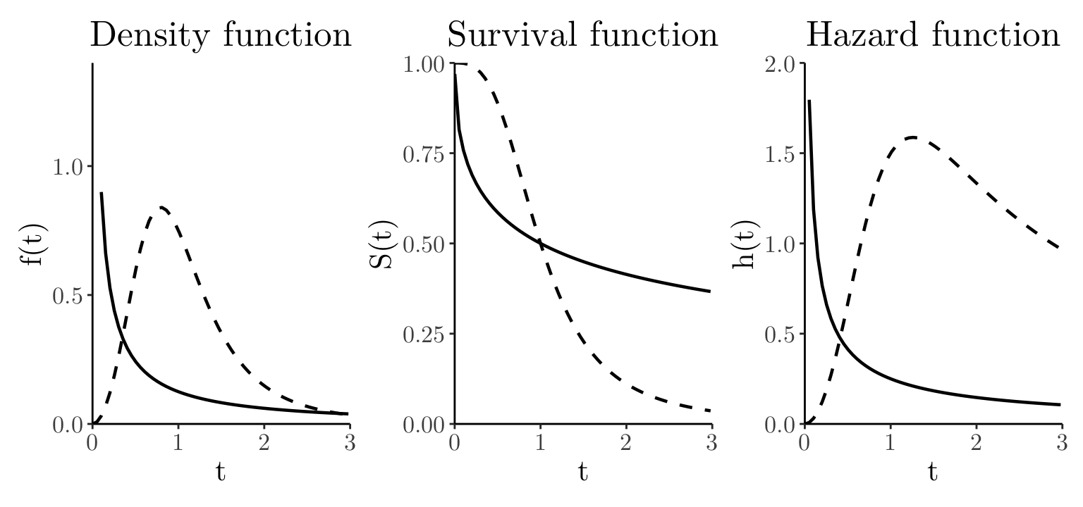
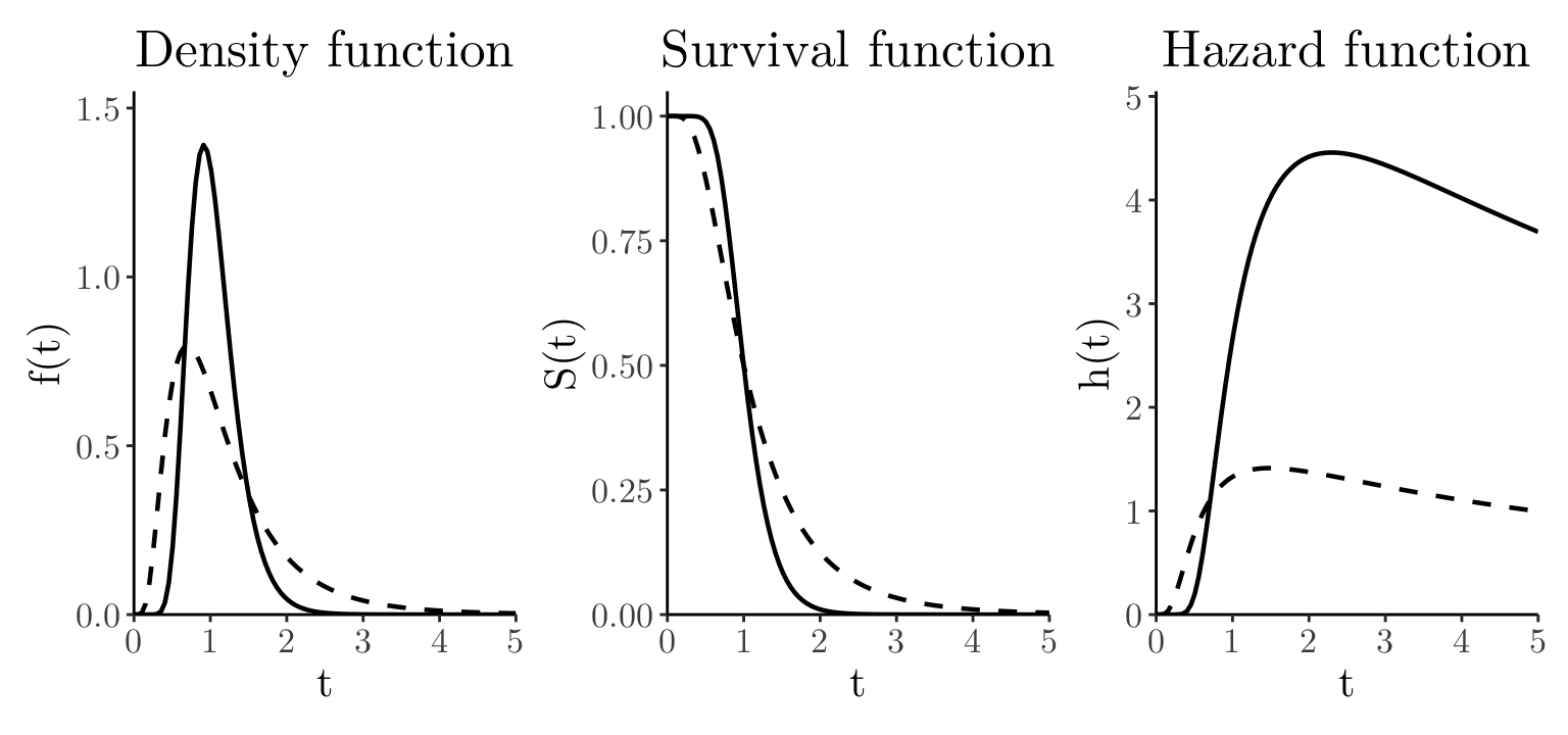
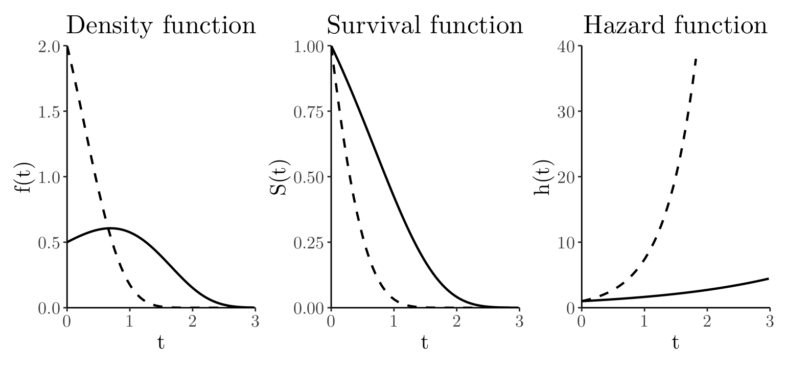
# The Log-Normal distribution has a *non-monotonic* hazard function that *rises rapidly* to a peak before *steadily decreasing* toward zero over time.
# E.g., initial high risk (electric components): chips immediately after production often contain latent manufacturing defects. These weak units fail quickly during the first few hours or days of operation. Once these defective chips have failed, the remaining units are considered "healthy," and their risk of failure decreases steadily toward zero.
t_seq <- seq(from = 0.001, to = 5, length.out = 100); sigma_values <- c(0.3, 0.6); mulog_scale <- 0 
df_combined <- lapply(sigma_values, function(sigma) { data.frame(t = t_seq, sigma_factor = factor(paste0("sigma = ", sigma)), ft = dlnorm(t_seq, meanlog = mulog_scale, sdlog = sigma), St = 1 - plnorm(t_seq, meanlog = mulog_scale, sdlog = sigma), ht = dlnorm(t_seq, meanlog = mulog_scale, sdlog = sigma) / (1 - plnorm(t_seq, meanlog = mulog_scale, sdlog = sigma))) }) %>% bind_rows()
custom_theme <- theme_bw() + theme(panel.grid.major = element_blank(), panel.grid.minor = element_blank(), panel.border = element_blank(), axis.line.x = element_line(linewidth = 0.5, color = "black"), axis.line.y = element_line(linewidth = 0.5, color = "black"), text = element_text(size = 16, family = "Latin Modern Roman 10"), legend.position = "right", legend.title = element_blank(), plot.title = element_text(hjust = 0.5))
shared_linetype <- scale_linetype_manual(values = c("sigma = 0.3" = "solid", "sigma = 0.6" = "dashed"))
p1 <- ggplot(df_combined, aes(x = t, y = ft, linetype = sigma_factor)) + geom_line(linewidth = 0.8) + labs(x = "t", y = "f(t)", title = "Density function" ) + shared_linetype + scale_x_continuous(limits = c(0, 5), expand = expansion(mult = c(0, 0))) + scale_y_continuous(limits = c(0, 1.55), expand = expansion(mult = c(0, 0))) + custom_theme + theme(legend.position = "none")
p2 <- ggplot(df_combined, aes(x = t, y = St, linetype = sigma_factor)) + geom_line(linewidth = 0.8) + labs(x = "t", y = "S(t)", title = "Survival function") + shared_linetype + scale_x_continuous(limits = c(0, 5), expand = expansion(mult = c(0, 0))) + scale_y_continuous(limits = c(0, 1.05), expand = expansion(mult = c(0, 0))) + custom_theme + theme(legend.position = "none")
p3 <- ggplot(df_combined, aes(x = t, y = ht, linetype = sigma_factor)) + geom_line(linewidth = 0.8) + labs(x = "t", y = "h(t)", title = "Hazard function"  ) + shared_linetype + scale_x_continuous(limits = c(0, 5), expand = expansion(mult = c(0, 0))) + scale_y_continuous(limits = c(0, 5.05), expand = expansion(mult = c(0, 0))) + custom_theme + theme(legend.position = "none")
p1 + p2 + p3

Gompertz distribution

The Gompertz distribution has two parameters, the shape \(\alpha>0\) and the scale \(\beta>0\). It is denoted \({\rm Gompertz}(\alpha,\beta)\) and has p.d.f. \[ f_T(t)=\alpha \exp\left(\beta t-\frac{\alpha}{\beta}(e^{\beta t}-1)\right), \] survival function \[ S_T(t)=\exp\left(-\frac{\alpha}{\beta}(e^{\beta t}-1)\right), \] and hazard function \[ h_T(t)=\alpha \exp(\beta t). \]

See Exercise 4 and 5 on Problem Sheet 1 for derivations of the survival and hazard function.

The Gompertz distribution models the idea that the instantaneous risk of death increases exponentially with age. For example, it can be used to model human lifetime from middle age onwards.

Gompertz distribution

The plots below show \(f(t)\), \(S(t)\), and \(h(t)\) for two different Gompertz distributions given by different values of \(\alpha\) (\(\text{solid} = 0.5\) and \(\text{dashed} = 2.0\)) but all with \(\beta = 1\).

t_seq <- seq(from = 0.001, to = 5, length.out = 100); beta_values <- c(0.5, 2); alpha_scale <- 1 # Assuming alpha=1
df_combined <- lapply(beta_values, function(beta) { data.frame(t = t_seq, beta_factor = factor(paste0("beta = ", beta)), ft = dgompertz(t_seq, shape = alpha_scale, rate = beta), St = 1 - pgompertz(t_seq, shape = alpha_scale, rate = beta), ht = alpha_scale * exp(beta * t_seq)) }) %>% bind_rows()
custom_theme <- theme_bw() + theme(panel.grid.major = element_blank(), panel.grid.minor = element_blank(), panel.border = element_blank(), axis.line.x = element_line(linewidth = 0.5, color = "black"), axis.line.y = element_line(linewidth = 0.5, color = "black"), text = element_text(size = 16, family = "Latin Modern Roman 10"), legend.position = "right", legend.title = element_blank(), plot.title = element_text(hjust = 0.5))
shared_linetype <- scale_linetype_manual(values = c("beta = 0.5" = "solid", "beta = 2" = "dashed"))
p1 <- ggplot(df_combined, aes(x = t, y = ft, linetype = beta_factor)) + geom_line(linewidth = 0.8) + labs(x = "t", y = "f(t)", title = "Density function" ) + shared_linetype + scale_x_continuous(limits = c(0, 3), expand = expansion(mult = c(0, 0))) + scale_y_continuous(limits = c(0,  2), expand = expansion(mult = c(0, 0))) + custom_theme + theme(legend.position = "none")
p2 <- ggplot(df_combined, aes(x = t, y = St, linetype = beta_factor)) + geom_line(linewidth = 0.8) + labs(x = "t", y = "S(t)", title = "Survival function") + shared_linetype + scale_x_continuous(limits = c(0, 3), expand = expansion(mult = c(0, 0))) + scale_y_continuous(limits = c(0,  1), expand = expansion(mult = c(0, 0))) + custom_theme + theme(legend.position = "none")
p3 <- ggplot(df_combined, aes(x = t, y = ht, linetype = beta_factor)) + geom_line(linewidth = 0.8) + labs(x = "t", y = "h(t)", title = "Hazard function"  ) + shared_linetype + scale_x_continuous(limits = c(0, 3), expand = expansion(mult = c(0, 0))) + scale_y_continuous(limits = c(0, 40), expand = expansion(mult = c(0, 0))) + custom_theme + theme(legend.position = "none")
p1 + p2 + p3