Survival Models (MATH3085/6143)

Chapter 3: The Survival Distribution

André Victor Ribeiro Amaral

a.v.ribeiro-amaral@soton.ac.uk

University of Southampton

29/09/2025

Recap

In the last chapter, we

• Defined statistical models in the context of survival analysis.
• Discussed using simplifying assumptions like independence and, sometimes, identical distribution (i.i.d.) to specify models.
• Differentiated between fully specified, parametric (parameters estimated from data), and non-parametric models.
• Introduced regression models, where differences in survival time distributions are explained by explanatory variables (covariates).

Chapter 3: The Survival Distribution

The density function (Gap on page 14)

We model survival time using a random variable \(T\).

If \(T\) is a continuous random variable (as we shall generally assume throughout this module), then its distribution is defined by its probability density function (p.d.f.) \(f_T(t)\), or \(f(t)\) for short.

Recall that, for any values \(t_1\) and \(t_2\), we have \[ \mathbb{P}(t_1\le T\le t_2)=\int_{t_1}^{t_2} f_T(t) \mathrm{d}t \]

The density function (Gap on page 14)

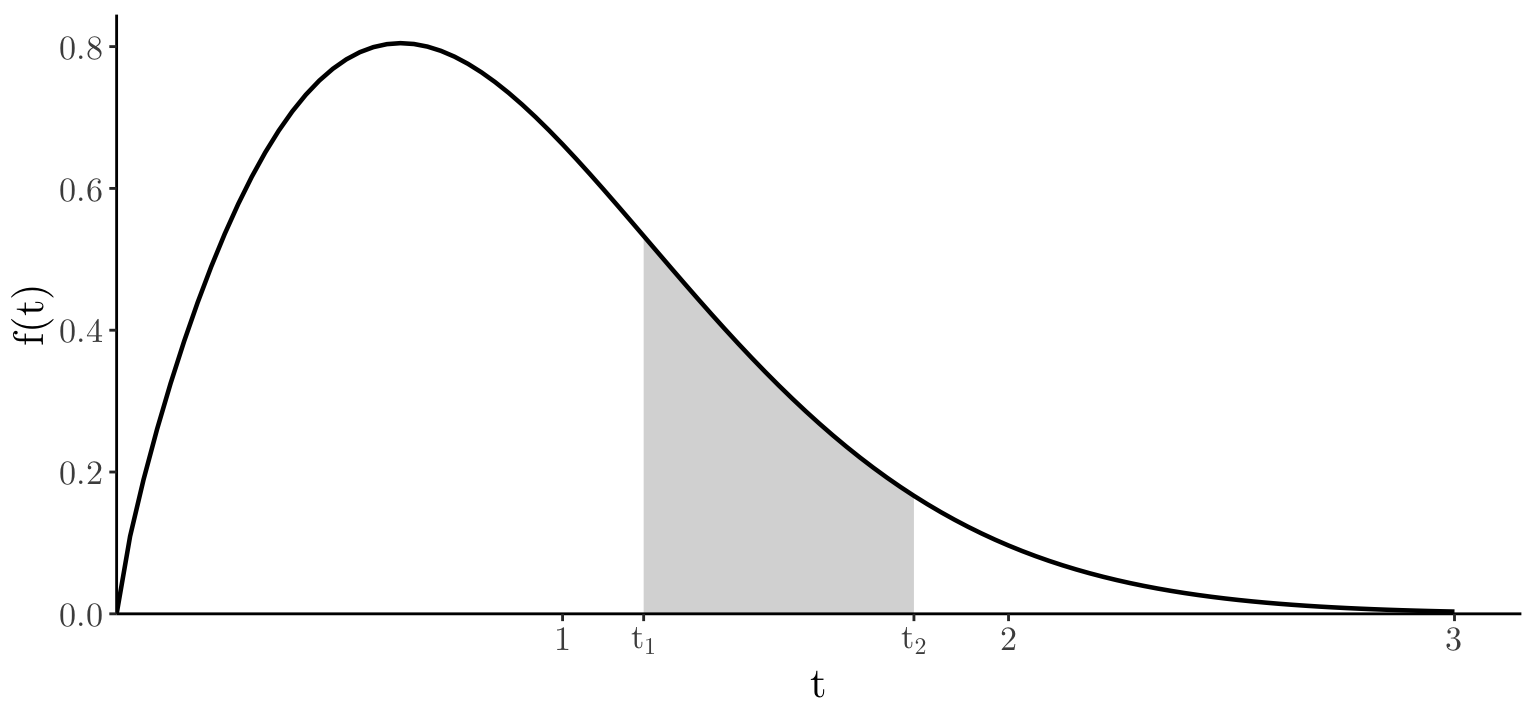
x_seq <- seq(0, 3, length = 100); df <- data.frame(t = x_seq, ft = dweibull(x_seq, 1.8, 1))

t1_val <- df[['t']][40]; t2_val <- df[['t']][60]

df_shade  <- filter(df, t >= t1_val & t <= t2_val); poly_data <- data.frame(t = c(t1_val, df_shade[['t']], t2_val), ft = c(0, df_shade[['ft']], 0))

ggplot(df, aes(x = t, y = ft)) +
  geom_polygon(data = poly_data, fill = "gray", alpha = 0.6) +
  geom_line(linewidth = 0.8) +
  theme_bw() +
  theme(panel.grid.major = element_blank(), panel.grid.minor = element_blank(), panel.border = element_blank(), axis.line.x = element_line(linewidth = 0.5, color = "black"), axis.line.y = element_line(linewidth = 0.5, color = "black")) +
  labs(x = "t", y = "f(t)") +
  scale_x_continuous(expand = expansion(mult = c(0, 0.05)), breaks = c(1, t1_val, t2_val, 2, 3), labels = c(1, expression(t[1]), expression(t[2]), 2, 3)) + scale_y_continuous(expand = expansion(mult = c(0, 0.05))) +
  theme(text = element_text(size = 16, family = "Latin Modern Roman 10"))

The distribution function (Gap on page 15)

Recall that the distribution function \(F_T(t)\), for a random variable \(T\), is defined as \[ F_T(t)=\mathbb{P}(T\le t) \] and that for a continuous survival (non-negative) variable with p.d.f. \(f_T\), we have \[ F_T(t)=\int_0^t f_T(s) \mathrm{d}s \]

The distribution function (Gap on page 15)

x_seq <- seq(0, 3, length.out = 100); df <- data.frame(t = x_seq, F_t = pweibull(x_seq, 1.8, 1))

ggplot(df, aes(x = t, y = F_t)) +
  geom_line(linewidth = 0.8) +
  geom_hline(yintercept = 1, linetype = "dashed", linewidth = 0.5) +
  theme_bw() +
  theme(panel.grid.major = element_blank(), panel.grid.minor = element_blank(), panel.border = element_blank(), axis.line.x = element_line(linewidth = 0.5, color = "black"), axis.line.y = element_line(linewidth = 0.5, color = "black")) +
  labs(x = "t", y = "F(t)") +
  scale_x_continuous(expand = expansion(mult = c(0, 0.0))) + scale_y_continuous(expand = expansion(mult = c(0, 0.05)), limits = c(0, 1)) +
  theme(text = element_text(size = 16, family = "Latin Modern Roman 10"))

The survival function (Gap on page 16)

In survival analysis, we usually prefer to focus on the survival function (sometimes called the survivor function), \(S_T(t)\), which is defined as \[ S_T(t)=\mathbb{P}(T> t) \] so for a continuous survival variable with p.d.f. \(f_T\), we have \[ S_T(t)=\int_t^\infty f_T(s) \mathrm{d}s \]

The survival function (Gap on page 16)

x_seq <- seq(0, 3, length.out = 100); df <- data.frame(t = x_seq, S_t = 1 - pweibull(x_seq, 1.8, 1))

ggplot(df, aes(x = t, y = S_t)) +
  geom_line(linewidth = 0.8) +
  geom_hline(yintercept = 0, linetype = "dashed", linewidth = 0.5) +
  theme_bw() +
  theme(panel.grid.major = element_blank(), panel.grid.minor = element_blank(), panel.border = element_blank(), axis.line.x = element_line(linewidth = 0.5, color = "black"), axis.line.y = element_line(linewidth = 0.5, color = "black")) +
  labs(x = "t", y = expression(S(t))) +
  scale_x_continuous(expand = expansion(mult = c(0, 0.0))) +  scale_y_continuous(expand = expansion(mult = c(0, 0.05)), limits = c(0, 1)) +
  theme(text = element_text(size = 16, family = "Latin Modern Roman 10"))

The survival function: properties (Gap on page 17)

• The survival function is a decreasing function of \(t\) with \(S_T(0) = 1\) and \(S_T(t) \to 0\) as \(t\to\infty\).

• The survival function is related to the distribution function through \[ S_T(t)+F_T(t)=1\qquad\Rightarrow\qquad S_T(t)=1-F_T(t) \]

• The expected lifetime is given, in terms of the survival function by \[ \begin{eqnarray*} \mathbb{E}(T) & = & \int_0^{\infty} u f_T(u) \mathrm{d}u\\ & = & \left[ - u S_T(u) \right]_0^\infty + \int_0^\infty S_T(u) \mathrm{d}u = \int_0^\infty S_T(t)dt, \end{eqnarray*} \] i.e., the area under the survival function curve.

The residual survival function (Gap on page 18)

The residual survival function is defined for \(t\ge 0\) as \[ S_T(t|x)=\mathbb{P}(T> t+x|T>x) \] for some specified \(x\). It gives the probability of surviving beyond \(t+x\) given that you have survived past \(x\).

It defines the distribution of future (beyond \(x\)) survival for the subpopulation of survivors up to time \(x\).

Using the standard definition of a conditional probability, we have \[ \begin{eqnarray*} S_T(t|x)&=&\frac{\mathbb{P}(T>t+x \quad \mbox{and} \quad T>x)}{\mathbb{P}(T>x)}\\[5pt] &=&\frac{\mathbb{P}(T>t+x)}{\mathbb{P}(T>x)}\\ &=&\frac{S_T(t+x)}{S_T(x)} \end{eqnarray*} \] Similarly the residual distribution function is \(F_T(t|x)=1-S_T(t|x)\).

The hazard function

The hazard function, \(h_T(t)\), represents the instantaneous rate of occurrence of the event (failure) at time \(t\), conditional on survival up to \(t\).

Note

Think of it as the answer to this question

If an individual is still alive at time \(t\), how likely are they to experience the event in the very next moment?

The hazard function (Gap on page 19)

The hazard function is defined for \(t\ge 0\) as \[ h_T(t) = \lim_{\delta t\to 0}\frac{\mathbb{P}(T\le t+\delta t|T> t)}{\delta t}. \] The numerator \(\mathbb{P}(T\le t+\delta t|T> t)\) can be thought of as the expected number of events in the time interval \((t,t+\delta t]\) (in a residual population of size \(1\) at time \(t\)).

Hence, the ratio

\[ \frac{\mathbb{P}(T\le t+\delta t|T> t)}{\delta t} \]

is the event rate over the time interval \((t,t+\delta t]\).

The hazard function is the limiting (or instantaneous) event rate at time \(t\).

The hazard function: properties (Gap on page 20)

The hazard function is given by

\[ \begin{eqnarray*} h_T(t) & = & \lim_{\delta t\to 0}\frac{\mathbb{P}(T\le t+\delta t|T> t)}{\delta t}\\ & = & \lim_{\delta t\to 0} \frac{ \mathbb{P}(T\le t+\delta t \quad \mbox{and} \quad T> t)}{\delta t \mathbb{P}(T> t)}\\ & = & \lim_{\delta t\to 0} \frac{ \mathbb{P}(t < T\le t+\delta t)}{\delta t \mathbb{P}(T> t)}\\ & = & \lim_{\delta t\to 0} \frac{ f_T(t) \delta t}{\delta t \mathbb{P}(T> t)} = \frac{ f_T(t)}{S_T(t)}. \end{eqnarray*} \]

The only constraint on the hazard function \(h_T(t)\) is that it must be non-negative for \(t\in (0,\infty)\).

hazard vs. density

• The hazard function
  • Compares the relative probabilities of events occurring at different times \(t\), conditional on \(T>t\).
  • Accounts for the size of the population at risk at \(t\) (i.e., the hazard only considers individuals who are still “at risk” at time \(t\), so it automatically adjusts for the shrinking number of people remaining in the population as time goes on.)

• The density function

  • Simply compares the relative probabilities of events occurring at different times \(t\) in the population at large.

• A time \(t\) with a high value for \(h(t)\) is not necessarily a likely failure time, as there may be a small probability that any individual survive until then.

hazard vs. density (Shiny App)

The integrated hazard function (Gap on page 21)

The integrated (cumulative) hazard function is defined by \[ H_T(t)=\int_0^t h_T(u) du. \] The integrated hazard function describes the total exposure to risk for a survivor up to \(T=t\).

Note that

\[ H_T(t)=\int_0^t h_T(u) du = \int_0^t \frac{f_T(u)}{S_T(u)} \mathrm{d}u. \]

Using the substitution \(v = 1/S_T(t)\), we have

\[ \frac{\mathrm{d}v}{\mathrm{d}u} = \frac{f_T(u)}{S_T(u)^2} \implies \mathrm{d}u = \frac{\mathrm{d}v S_T(u)^2}{f_T(u)}. \]

Then, \[ H_T(t) = \int_1^{1/S_T(t)} \frac{1}{v} \mathrm{d}v = \left[ \log v \right]_1^{1/S_T(t)} = - \log S_T(t). \]

Relationships

• Only one of the functions \(f_T\), \(F_T\), \(S_T\), \(h_T\), or \(H_T\) needs to be specified to completely determine the distribution of \(T\).

• In survival analysis, interest is usually focused on the survival function \(S_T(t)\) and the hazard function \(h_T(t)\).

	\[f_T\]	\[S_T\]	\[h_T\]
\[f_T(t) = \]		\[-\frac{\mathrm{d}}{\mathrm{d}t} S_T(t)\]	\[h_T(t)\exp\left[-\int_0^t h_T(s)\mathrm{d}s\right]\]
\[S_T(t) = \]	\[\int_t^\infty f_T(s)\mathrm{d}s\]		\[\exp\left[-\int_0^t h_T(s)\mathrm{d}s\right]\]
\[h_T(t) = \]	\[\frac{f_T(t)}{\int_t^\infty f_T(s)\mathrm{d}s}\]	\[-\frac{\mathrm{d}}{\mathrm{d}t} \log S_T(t)\]