# A tibble: 33 × 3
     wbc ag       time
   <int> <fct>   <int>
 1  2300 present    65
 2   750 present   156
 3  4300 present   100
 4  2600 present   134
 5  6000 present    16
 6 10500 present   108
 7 10000 present   121
 8 17000 present     4
 9  5400 present    39
10  7000 present   143
# ℹ 23 more rowsSurvival Models (MATH3085/6143)
Chapter 2: Statistical Models
20/10/2025
Recap
In the last chapter, we
- Learned that survival analysis is a field dedicated to analyzing time-to-event data.
- Identified the challenges in working with time-to-event data, such as censoring and truncation.
- Defined censoring as having incomplete information about a subject’s event time.
- Defined truncation as having incomplete information about the group of people being studied.
Chapter 2: Statistical Models
Introduction
Statistical analysis (or inference) involves
- Drawing conclusions and
- Making decisions and predictions
using the evidence provided to us by observed data.
To do this, we use statistical models, where we simulate the process by which the observed data were generated through a probability distribution.
Introduction
- The form of the model helps us to understand the real-world process by which the data were generated.
- If the model explains the observed data well, then it should also inform us about future (or unobserved) data, and hence help us to make predictions (and decisions).
- The use of statistical models also allows us to quantify the uncertainty associated with any conclusions, predictions or decisions we make.
We rarely believe in our models, but regard them as temporary constructs subject to improvement.
Example: Leukaemia
Survival times are given for 33 patients who died from acute myelogenous leukaemia. In R, this can be found in the leuk object in the MASS package.
leuk is a data frame with columns: wbc (white blood count), ag (a test result, “present” or “absent”), and time (survival time in weeks).
Notation
- Suppose that we have \(n\) data observations, then we use \[ t_1,t_2,\cdots , t_n \] to denote these observed event (failure, death, \(\cdots\)) or censoring times.
- For the leukaemia survival times, \(n=33\) and \(t_1=65\), \(t_2=156\), \(\cdots , t_{33}=43\).
- We denote the complete data by the vector \(\mathbf{t}=(t_1,t_2, \cdots , t_n)\).
Notation
- In a statistical model, we consider \(t_1,t_2, \cdots , t_n\) to be observations of random variables (denoted with the corresponding capital letters) \[ T_1,T_2,\cdots , T_n. \]
- We also use the vector notation \(\mathbf{T}=(T_1,T_2,\cdots , T_n)\).
This is the same as MATH2010, but with \(t\) and \(T\), instead of \(y\) and \(Y\), respectively.
Statistical models
A statistical model specifies a probability distribution for the random variables \(\mathbf{T}\) corresponding to the data observations \(\mathbf{t}\).
Providing a specification for the distribution of \(n\) jointly varying random variables is made much easier if we can make some simplifying assumptions, such as
- \(T_1,T_2,\cdots , T_n\) are independent random variables.
- \(T_1,T_2,\cdots , T_n\) have the same probability distribution (so \(t_1,t_2, \cdots , t_n\) are observations of a single random variable \(T\)).
Statistical models
- \(T_1,T_2,\cdots , T_n\) are independent random variables.
- \(T_1,T_2,\cdots , T_n\) have the same probability distribution (so \(t_1,t_2, \cdots , t_n\) are observations of a single random variable \(T\)).
Assumption 1 is very common, even in quite complex examples.
Assumption 2 is not always appropriate, but may be reasonable when we are modelling a homogeneous population, without other information.
- Making assumption
2means we cannot include explanatory variables, so sometimes we will not make this assumption.
When we make assumptions 1 and 2, we say that \(T_1,T_2,\cdots , T_n\) are independent and identically distributed (i.i.d.).
A fully specified model
Sometimes a model completely specifies the probability distribution of \(T_1,T_2,\cdots , T_n\).
For example, for the leukaemia survival times, we might assume the model
\[ T_1,T_2,\ldots , T_n \stackrel{\text{i.i.d.}}{\sim} \mathrm{lognormal}(\mu,\sigma^2) \] where \(\mu=3\) and \(\sigma^2=4\).
Note that \(T_1,T_2,\cdots , T_n \stackrel{\text{i.i.d.}}{\sim} \mathrm{lognormal}(\mu,\sigma^2)\) is equivalent to \[ \log(T_1), \log(T_2), \cdots , \log(T_n) \stackrel{\text{i.i.d.}}{\sim} \mathrm{N}(\mu,\sigma^2), \] where \(\log\) is the natural logarithm.
A fully specified model
For example, for the leukaemia survival times, we might assume the model \[ T_1,T_2,\cdots , T_n \stackrel{\text{i.i.d.}}{\sim} \mathrm{lognormal}(\mu,\sigma^2) \] where \(\mu=3\) and \(\sigma^2=4\).
- The key is that we have assumed exact values for \(\mu\) and \(\sigma^2\).
- This would be appropriate when there is some external (to the data) theory as to why the model (in particular \(\mu=3\) and \(\sigma^2=4\)) is appropriate.
- The data can then be used to assess the plausibility of the model. Do the data support the model or not?
- We rarely have external theory to specify a model so precisely.
A parametric statistical model
For the leukaemia survival times, a more common model would be \[ T_1,T_2,\cdots , T_n \stackrel{\text{i.i.d.}}{\sim} \mathrm{lognormal}(\mu,\sigma^2) \] where \(\mu\) and \(\sigma^2\) are unspecified.
This is called a parametric statistical model as it completely specifies the probability distribution which generated the data, apart from a (small) number of parameters (here \(\mu\) and \(\sigma^2\)).
The data are then used to estimate the unknown parameters (\(\mu\) and \(\sigma^2\)), and to assess the plausibility of other assumptions (lognormal distribution, independence, etc.).
A non-parametric statistical model
Sometimes, it is not appropriate, or we want to avoid, making a precise specification for the distribution which generated \(T_1,T_2,\cdots , T_n\).
Then, we might propose the model \[ T_1,T_2,\cdots , T_n \text{ are i.i.d. random variables.} \]
This is sometimes described as a nonparametric (or distribution-free) specification.
A non-parametric statistical model
It imposes limitations on the kind of statistical inferences we can obtain, but still allows us to do some interesting things, such as the following
- Use exploratory/graphical techniques, such as box plots and histograms to learn about the distribution of the (common) random variable \(T\) which generated the data.
- Estimate features of the distribution of \(T\), such as its expectation \(\mathbb{E}(T)\), variance \(\text{Var}(T)\), \(\mathbb{P}(T>t_0)\) for some specified \(t_0\), etc.
- Estimate the distribution or survival function of \(T\) (to be covered in this module).
Regression models
Often, we model survival data to learn about the relationship between survival time \(T\) and other potentially explanatory variables \(x_1,x_2, \cdots\).
The leukaemia survival times include values of two such explanatory variables
ag, taking values in the set \(\left\{\mathrm{present},~\mathrm{absent}\right\}\) (a test result).wbc(white blood cell count), a numerical variable.
Common assumptions
- \(T_1,T_2,\cdots , T_n\) are independent random variables.
- \(T_1,T_2,\cdots , T_n\) have the same probability distribution (so \(t_1,t_2, \cdots , t_n\) are observations of a single random variable \(T\)).
In a regression model, we assume that \(T_1 ,T_2,\cdots , T_n\) are independent random variables but they are not identically distributed (we make assumption 1 but not assumption 2).
Regression models
Instead, we assume the differences between their distributions is explained by a regression function of the values of the explanatory variables.
For example, for \(i=1,\cdots,n\) we assume \(T_i \sim \mathrm{lognormal}(\mu_i,\sigma^2)\) independently with \[
\mu_i=\beta_0+\beta_1 x_{i1} +\beta_2 x_{i2}
\] where \(x_{i1}\) is the \(i\)-th value of wbc and \[
x_{i2} =
\left\{ \begin{array}{ll}
1 & \text{if}~~\texttt{ag}~~\text{is present}\\
0 & \text{if}~~\texttt{ag}~~\text{is absent}
\end{array}
\right.
\] i.e., \(x_{i2}\) is a dummy variable.
The data analysis process
The data analysis can be summarised by the following diagram
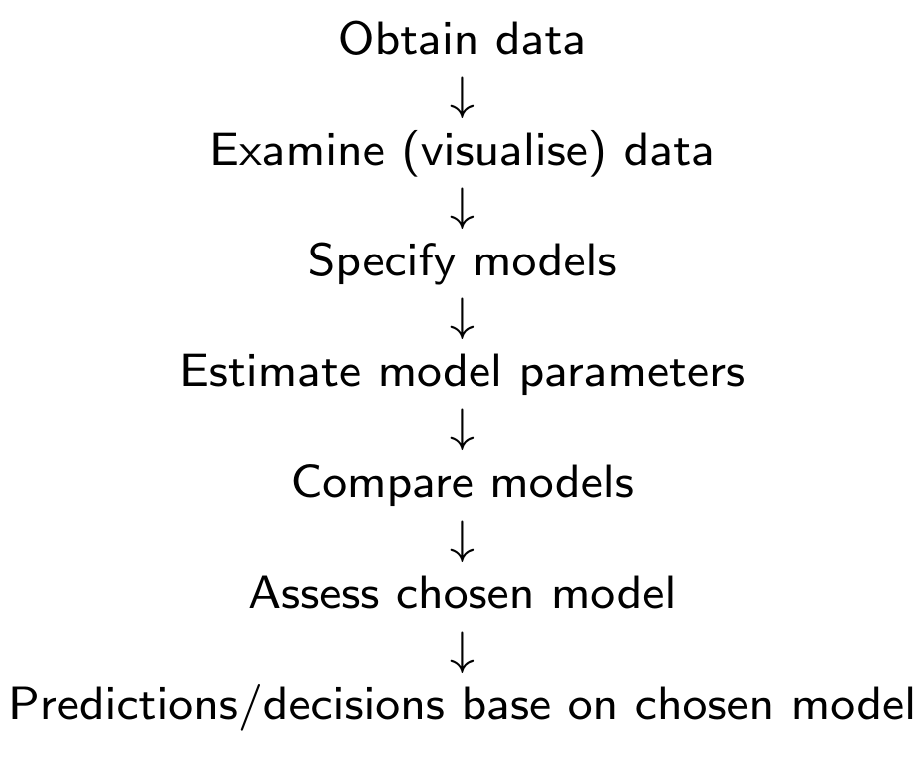
In MATH3085/6143, we focus on models and methods which have been specifically developed for survival data.