Survival Models (MATH3085/6143)

Chapter 1: Introduction

André Victor Ribeiro Amaral

a.v.ribeiro-amaral@soton.ac.uk

University of Southampton

30/09/2025

Preface

These slides are based on material written by previous lecturers of this course.

Information about the module (syllabus, schedule, etc.) is available on Blackboard and on the module website (avramaral.github.io/MATH3085/).

Instructors

This module will be co-taught by

1. Dr André Amaral (a.v.ribeiro-amaral@soton.ac.uk): Chapters 1-9
2. Dr Chao Zheng (chao.zheng@southampton.ac.uk): Chapters 10-16

For any queries, please see either of us during our office hours

• Dr André Amaral (weeks 1-6): Tuesday, 14:00–16:00, Room 54/10007.
• Dr Chao Zheng (weeks 7-11 and 15): Tuesday, 14:00–16:00, Room 54/9001.

Timetabling

MATH3085/6143 has been given a timetable with the following slots

Day	Time	Room
Tuesday	16:00–18:00	02/1089
Thursday	15:00–17:00	35/1001

Below is the tentative schedule for the first part of the module.

Week	Tuesday (Session 1)	Tuesday (Session 2)	Thursday (Session 1)	Thursday (Session 2)
01	Chapter 1	Chapter 2	Chapter 3	Chapter 4 (part 1)
02	Chapter 4 (part 2)	Problem Sheet 1	Chapter 5	Chapter 6 (part 1)
03	Chapter 6 (part 2)	Chapter 6 (part 3)	Chapter 6 (part 4)	Problem Sheet 2
04	Chapter 7 (part 1)	Chapter 7 (part 2)	Chapter 7 (part 3)	Problem Sheet 3
05	Chapter 8 (part 1)	Chapter 8 (part 2)	Chapter 8 (part 3)	Chapter 8 (part 4)
06	Chapter 9 (part 1)	Chapter 9 (part 2)	Chapter 9 (part 3)	Problem Sheet 4

How is MATH3085/6143 taught?

• Lecture
  • Slides and video recordings can be downloaded after every lecture.
  • Lecture notes are available in two formats (skeleton & complete).

• Problem Class
  • Will work through 6 problem sheets.
  • Please attempt the problems before the problem class.
  • Solutions will be available after the problem class.

• R Self-paced Tutorial
  • Do not need to start until after Chapter 7.
    
  • Drop-in support for R (details to be released later).

Assessment

The basic module assessment breakdown is

1. 30% data analysis project
2. 70% written exam

The data analysis project involves a series of tasks in which you will conduct survival analysis on provided datasets using R. The project will be released around mid-December 2025, and detailed instructions and guidance will be provided towards the end of the term.

Chapter 1: Introduction

Survival Analysis

• The aim in most statistical modelling problems (e.g. MATH2010) is to investigate the relationship between
  • an observed response (usually denoted by \(y\)) .
  • \(k\) explanatory variables (denoted by \(x = (x1, \cdots, x_k)\)).

• In MATH3085/6143, the response is always the time from origin until an event of interest occurs.

• Because the response is a time, we denote the observation using \(t\), and the corresponding random variable using \(T\).
  

Survival Analysis

Survival analysis refers to a set of special statistical methods required to analyse time-to-event data.

The object of survival modelling is to learn about the variability in \(T\) in a population of interest and (often) how this is associated with other potentially explanatory variables (covariates).

Applications and alternative terminology

Historically, survival analysis originated from medical applications where

• the event was death, and
• the time to the event was called the survival time.

Sir David Cox (1924–2022) and his seminal paper in 1972.

Applications and alternative terminology

However, survival analysis now has applications in many areas beyond medicine including the following

• Demography: age at “milestone,” such as
  • death,
  • birth of first child, etc.

• Engineering
  • failure time of a machine.

• Economics
  • duration of unemployment.

• Psychology
  • response time to stimulus or activation.

Applications and alternative terminology

Important actuarial examples where we are required to model survival data include

• Time between pensionable age and death.

• Time between taking out a life insurance policy and death.

• Time between taking out a critical illness insurance policy and onset of illness.

• Failure time for a product with warranty insurance.

Applications and alternative terminology

Due to the different application areas, you may encounter different terminologies.

The following table summarises alternative terminologies you may encounter in this module and elsewhere.

Survival analysis	Origin	Event of interest	Time to event
Event history analysis	Initial event	Death	Survival time
Duration analysis	Initiating event	Failure	Failure time
Hazard modelling	Starting event	Endpoint	Response time
Reliability analysis	Time origin	Outcome	Waiting time
		Terminating event	Duration
		Target event	Spell
			Episode

Why is Survival Analysis “special”?

Why does survival analysis need its own module?

• Models for non-negative random variable \(T\). In MATH2010, the response had a normal distribution which allows for negative responses.

• Data are often not well-described by standard probability distributions, e.g. the normal distribution.

• Data are typically censored (explained soon).

• Model parameters often not of primary interest. Often interest in the whole survival distribution, e.g. all quantiles, not just measures of location such as mean or median.

• Time-dependent covariates, i.e. they are not fixed like in MATH2010.

• Truncation: some cases may be missing (explained soon).

Types of time to event

• Continuous time
  • In theory, the value of \(T\) can be recorded to arbitrary precision.
    
  • In practice, the value of \(T\) is rounded to a convenient level of precision.
    
  • Tied data values cannot occur in theory (with probability 0), but do in practice.

• Grouped continuous time
  • Imprecise time measurements, only reporting the interval in which the observation lies.
    
  • Example: time in completed years, months, weeks, or days.
    
  • Common in population mortality studies (report age in completed years at death).

• Discrete time
  • True discrete-time scale, \(T = 1, 2, 3, \cdots\).
  • Example: number of operations of a machine to first failure, number of attempts to pass a test, etc.

Censoring

A common feature of survival data is censoring.

• Censoring occurs when we do not know all times-to-event \(T\) exactly, but only have bounds on some of the survival times.

• Special methods are needed for censored data because
  • Censored observations provide information.
    
  • Exclusion of censored data leads to bias.
  • Discarding censored data would be inefficient.

Censoring

Observations of \(T\) may be

• observed precisely,
• right censored,
• left censored, or
• interval censored.

In statistical modelling, censoring has to be taken into account to avoid bias.

Right censoring (Gap on page 04)

An observation of \(T\) is right censored if we only observe a lower bound for \(T\), i.e. we know that \(T\) was greater than some value, e.g. \(18\), but not the exact value itself.

A censored value with be denoted by \(T^*\) or \(T^+\), so we know \[T \ge T^* \qquad \mbox{equivalently} \qquad T \in \left(T^*, \infty \right).\]

Right censoring

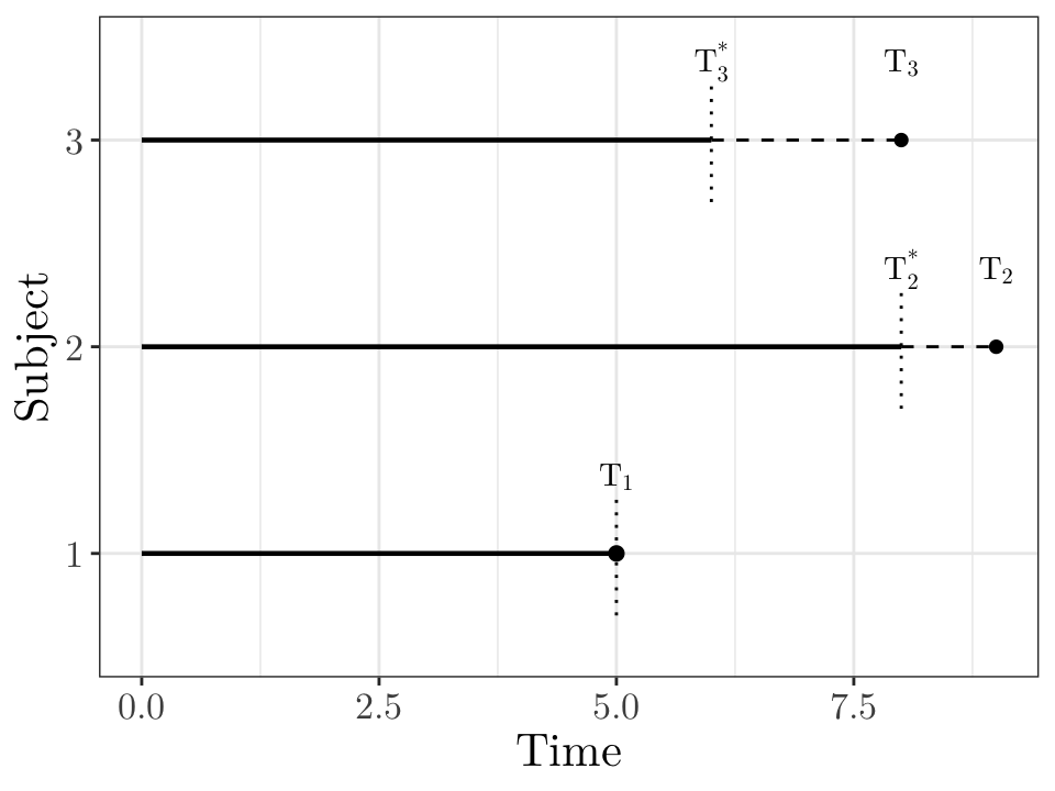
# In this figure, subject 1 is not censored and we would observe the response T_1. 
# Subjects 2 and 3 are right censored: we only know that the true responses T_2 and T_3 are greater than T_2^* and T_3^*, respectively.

d <- data.frame(id = c(1, 2, 3), start = c(0, 0, 0), end = c(5, 8, 6), added =  c(0, 1, 2), status = c(1, 0, 0))

p <- ggplot(d, aes(y = factor(id))) +
       geom_segment(aes(x = start, xend = end, yend = factor(id)), linewidth = 0.8, colour = "black") +
       geom_segment(aes(x = end, xend = end, y = as.numeric(factor(id)) - 0.3, yend = as.numeric(factor(id)) + 0.3), linetype = "dotted", colour = "black") +
       geom_point(data = filter(d, status == 1), aes(x = end, y = factor(id)), size = 2) +
       geom_segment(data = filter(d, status == 0), aes(x = end, xend = end + added, yend = factor(id)), linetype = "dashed", colour = "black") +
       geom_point(data = filter(d, status == 0), aes(x = end + added), size = 2, shape = 16, colour = "black") + 
       scale_y_discrete(name = "Subject", labels = c("1", "2", "3")) + scale_x_continuous(name = "Time") +
       theme_bw() + theme(text = element_text(size = 16, family = "Latin Modern Roman 10"))
p + annotate("text", x = 5.0, y = 1.18, label = "T[1]", vjust = -1, family = "Latin Modern Roman 10", parse = TRUE) + annotate("text", x = 8.0, y = 2.09, label = "T[2]^'*'", vjust = -1, family = "Latin Modern Roman 10", parse = TRUE) + annotate("text", x = 9.0, y = 2.18, label = "T[2]", vjust = -1, family = "Latin Modern Roman 10", parse = TRUE) + annotate("text", x = 6.0, y = 3.09, label = "T[3]^'*'", vjust = -1, family = "Latin Modern Roman 10", parse = TRUE) + annotate("text", x = 8.0, y = 3.18, label = "T[3]", vjust = -1, family = "Latin Modern Roman 10", parse = TRUE)

Right censoring

Reasons for right censoring include

• Event (e.g., death) has not been observed before the end of study;
• Individual lost-to-followup.
• Individual withdrawal from study.

In most survival analyses (particularly involving mortality) we should expect right censoring.

Left censoring

An observation of \(T\) is left censored if we only observe an upper bound for \(T\), i.e., we know that \(T\) was less than some value, e.g. \(18\), but not the exact value itself.

• Left censoring is not as common as right censoring.
• Example: a patient enrolls in a study for a chronic illness, but they already have the illness. You know the illness started before their enrollment date.

Interval censoring

An observation of \(T\) is interval censored if we only observe an interval for \(T\), i.e. we know that \(T\) is between two values, e.g. \((18,~ 20)\), but not the exact value itself.

• Note that left and right censored observations are actually interval censored where the upper or lower limit of the interval is \(-\infty\) or \(\infty\), respectively.
• Example (recurrence of a disease): a patient with cancer undergoes surgery. They are given a check-up at time \(t_1\) and show no signs of recurrence. At their next check-up at time \(t_2\), the cancer has returned. The event of recurrence is interval-censored between \(t_1\) and \(t_2\).

Informative and non-informative censoring

Censoring is informative if the reason for a subject being censored is related to their survival time \(T\). This means the censoring event itself provides extra information about the subject’s outcome beyond simply knowing that their survival time falls within a certain range.

Censoring is non-informative if the reason for a subject being censored is unrelated to their survival time (the standard assumption in most cases).

Informative and non-informative censoring

• Let \(T\) be the true time until the event of interest occurs. It is the survival time you would measure if you could follow a subject indefinitely.

• Let \(C\) be the time a subject is censored. It is when their observation ends for reasons other than the event itself.

In a survival study, we may have

• The event occurs first (\(T \leq C\)): if the event time \(T\) is less than or equal to the censoring time \(C\), you get to observe the event. You know the exact value of \(T\).
• Censoring occurs first (\(T > C\)): if the true event time \(T\) is greater than the censoring time \(C\), you do not get to see the event. You only know that the subject survived up to time \(C\). The observation is right-censored, and all you can say is that the true event time \(T\) is in the interval \((C, ~\infty)\).

Informative and non-informative censoring

Examples of causes of informative censoring include

• Patients lost to follow-up because of good prognosis.
• Withdrawals of patients due to ill health related to outcome of interest.

A sufficient condition for non-informative censoring is that \(C\) and \(T\) are independent variables. For example \(C\) is a (non-random) time fixed in advance of the study.

Informative censoring causes complications for statistical modelling because we need a joint model for \(T\) and \(C\). We will assume non-informative censoring throughout.

Truncation

Left truncation of survival data occurs when cases whose survival times \(T\) are shorter than a given time, either fixed or random, are not observed.

• Example: a study of heart attack survival which excludes individuals who died before reaching hospital.

Right truncation of survival data occurs when cases which have not experienced the event are not observed.

• Example: data obtained from death certificates (individuals who are still alive are not included in the sample).

The key difference between censoring and truncation is that censoring deals with incomplete information about the event time, while truncation deals with incomplete information about the group of people being studied.

Goals of survival analysis

Some basic goals of survival analysis include the following

• Describe how survival in the sample depends on time.

• Inference to the population of interest.

• Compare whole survival distributions for groups.

• Explain survival differentials using explanatory variables.

• Predict future survival.